
1. Introduction
The Theory of Consumer Behaviour explains how consumers allocate their limited income among goods and services to maximise satisfaction, or utility. It forms the foundation of microeconomic analysis and demand theory.
The central question is:
Given income and prices, what combination of goods will a rational consumer choose to maximise satisfaction?
2. Approaches to the Theory of Consumer Behaviour
A. Cardinal Utility Approach (Marshallian Approach)
Assumptions
- Measurable utility: Utility can be measured in cardinal numbers, such as 1, 2 and 3, expressed in units called utils.
- Rational consumer: The consumer aims to maximise total utility.
- Diminishing marginal utility: The additional utility derived from each extra unit of a good declines as consumption increases, other things remaining constant.
- Independent utilities: In the traditional additive model, the utility of one commodity is independent of the consumption of others.
- Constant marginal utility of money: The marginal utility of money remains unchanged during the analysis.
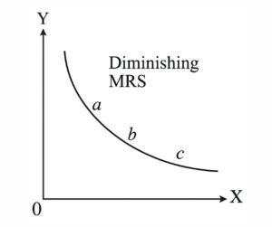
Law of Diminishing Marginal Utility (DMU)
As more units of a good are consumed, the additional satisfaction from each successive unit decreases, other things remaining constant.
- MUx: Marginal utility of good X.
- ΔTU: Change in total utility.
- ΔQx: Change in the quantity of X consumed.
Consumer’s Equilibrium under Cardinal Utility
For goods consumed in positive quantities, the consumer allocates income so that marginal utility per unit of money spent is equal across goods:
Here, Px and Py are prices, and MUm is the marginal utility of money. The allocation must also satisfy the consumer’s budget constraint.
B. Ordinal Utility Approach (Indifference Curve Analysis)
Key Contributors
Vilfredo Pareto contributed to ordinal utility theory. J. R. Hicks and R. G. D. Allen developed the approach in their 1934 work. Hicks further developed it in Value and Capital (1939).
Core Concept
Utility need not be measured numerically; preferences can be ranked. Consumers can compare bundles without stating exactly how much satisfaction each provides.
Assumptions of the Standard Model
- Rationality: The consumer seeks the most preferred affordable bundle.
- Completeness and ordinal ranking: The consumer can rank any two bundles or regard them as equally preferred.
- Transitivity: If A is preferred to B and B to C, then A is preferred to C.
- Non-satiation: More of a desirable good is preferred to less, other things remaining constant.
- Diminishing marginal rate of substitution: As X replaces Y, the consumer is willing to give up progressively less Y for an additional unit of X.
3. Indifference Curve Analysis
Indifference Curve (IC)
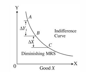
An indifference curve shows combinations of two goods that provide equal satisfaction. The consumer is indifferent among all bundles on the same curve.
Properties of Standard Indifference Curves
- Negatively sloped: For two desirable goods, gaining more of one requires giving up some of the other to maintain the same utility.
- Convex to the origin: This reflects diminishing MRS.
- Non-intersecting: Distinct indifference curves cannot cross under consistent preferences.
- Higher curves indicate higher utility: Under non-satiation, curves farther to the northeast represent more preferred bundles: IC3 > IC2 > IC1.
Exam note: Perfect substitutes have straight-line indifference curves; perfect complements have L-shaped curves. Smooth, strictly convex curves describe the standard case.
Marginal Rate of Substitution (MRS)
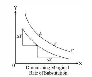
MRS is the amount of Y a consumer is willing to give up for an additional unit of X while keeping satisfaction constant.
The finite-change ratio approximates MRS over a segment. At a point on a smooth curve:
Diminishing MRS: As more X is consumed, less Y is sacrificed for each additional unit of X. This explains convexity to the origin.
Budget Line
The budget line represents combinations of X and Y that exactly exhaust income M at prices Px and Py. Affordable bundles lie on or below this line.
With X on the horizontal axis and Y on the vertical axis:
Shifts and Rotations
- Income increases, prices unchanged: Parallel outward shift.
- Income decreases, prices unchanged: Parallel inward shift.
- One price increases, income and the other price unchanged: Inward rotation around the unchanged intercept.
Consumer’s Equilibrium (Indifference Curve Approach)
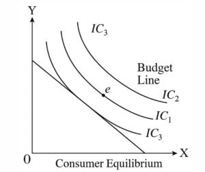
In the standard smooth, convex case, an interior equilibrium occurs where the highest attainable indifference curve is tangent to the budget line:
At equilibrium, the consumer maximises satisfaction subject to the budget constraint.
Exam note: Tangency is not universal. Corner solutions and kinked indifference curves require separate analysis.
4. Revealed Preference Theory (Samuelson)
Samuelson introduced the revealed preference approach in 1938. It examines observed choices instead of relying on directly measurable utility.
Assumptions and Consistency Conditions
- Choice from affordable bundles: The consumer selects a preferred bundle from the available budget set.
- Consistency: Choices should satisfy revealed preference restrictions.
- Stable preferences: Preferences are treated as unchanged across the observations being compared.
- Transitivity: A consistent ordering rules out preference cycles; stronger revealed preference conditions address chains of choices.
Axiom of Revealed Preference
If the consumer chooses A when B is also affordable, A is directly revealed preferred to B.
Under the usual single-valued choice formulation of the Weak Axiom of Revealed Preference (WARP), if A is chosen when B is affordable, B should not later be chosen when A is also affordable.
Implications
- Provides testable restrictions on observed demand behaviour without measuring utility.
- Supports the compensated law of demand under appropriate conditions. Uncompensated demand can still exhibit Giffen behaviour.
- With sufficiently rich data and appropriate consistency conditions, choices can be rationalised by preferences.
5. Theory of Consumer Surplus
Origin
The concept is associated with A. J. Dupuit (1844) and was later developed by Alfred Marshall.
Meaning
Consumer surplus is the difference between total willingness to pay for the units purchased and the amount actually paid.
Graphically, it is the area below the demand curve and above the market price, up to the quantity purchased.
Formula clarification: CS = TU − (P × Q) is meaningful only when total utility is expressed in money units. Utility measured in utils cannot be directly subtracted from monetary expenditure.
Hicksian Measurement
Hicks developed ordinal welfare measures using indifference curves and budget constraints. Compensating variation and equivalent variation express welfare changes in money while holding a specified utility level constant. They can differ from ordinary demand-curve consumer surplus when income effects matter.
6. Criticisms and Limitations
| Theory | Key limitations |
|---|---|
| Cardinal utility | Utility is difficult to measure objectively; constant marginal utility of money is a restrictive assumption. |
| Indifference curve analysis | Two-good diagrams simplify real choices; stable, consistent preferences may not capture all observed behaviour. |
| Revealed preference | Requires comparable choice observations and stable preferences; identifies choice patterns more readily than psychological motives. |
| Consumer surplus | Depends on willingness-to-pay estimates; ordinary demand-curve surplus may be an imperfect welfare measure when income effects are substantial. |
Consumer surplus can be applied to necessities, but estimating willingness to pay and interpreting welfare may be difficult.
7. Modern Developments in Consumer Behaviour
- Behavioural economics: Studies bounded rationality, heuristics, biases and departures from conventional choice assumptions.
- Expected utility and risk: Examines choices under uncertainty through probability-weighted utilities.
- Intertemporal choice: Examines consumption and saving across time, including Fisher’s model.
8. Key Diagrams for UGC NET
- Indifference curves and the budget line: consumer equilibrium.
- Diminishing marginal rate of substitution.
- Revealed preference and budget constraints.
- Hicksian welfare measures: compensating and equivalent variation.
9. Summary Points
- Consumer behaviour explains choices under income and price constraints.
- Cardinal utility assumes measurable satisfaction; ordinal utility requires only preference ranking.
- Indifference curve analysis identifies the most preferred affordable bundle.
- Revealed preference examines consistency through observed choices.
- Consumer surplus measures willingness to pay above expenditure, subject to measurement and welfare qualifications.
10. Suggested Readings
- Hicks, J. R. — Value and Capital.
- Samuelson, P. A. — Foundations of Economic Analysis.
- Dwivedi, D. N. — Principles of Economics.
- Mankiw, N. G. — Principles of Microeconomics.
- Koutsoyiannis, A. — Modern Microeconomics.
