Tag: UGC NET Economics exam expected question

UGC NET Economics Unit 1-Theory of Production and Costs MCQs-1

1.

The production function expresses:
A) A financial relationship between cost and output
B) The physical relationship between inputs and output
C) The functional relationship between price and output
D) The demand for factors of production
Answer: B

2.

In the short run, at least one factor of production is:
A) Variable
B) Fixed
C) Unavailable
D) Indivisible
Answer: B

3.

Which of the following best defines the law of variable proportions?
A) All inputs change in the same proportion
B) At least one input is fixed and one is variable
C) Returns increase indefinitely with input usage
D) Output remains constant despite input change
Answer: B

4.

In the law of variable proportions, diminishing returns occur because:
A) Technology improves
B) Fixed factors are overused
C) Variable inputs become cheaper
D) Inputs become more productive
Answer: B

5.

The Marginal Rate of Technical Substitution (MRTS) measures:
A) How much capital substitutes for labour keeping cost constant
B) The rate at which one input substitutes another keeping output constant
C) The ratio of marginal products to total cost
D) The ratio of input prices
Answer: B

6.

Which of the following statements about isoquants is correct?
A) Isoquants slope upward to the right
B) Higher isoquants show lower levels of output
C) Isoquants are convex to the origin due to diminishing MRTS
D) Isoquants can intersect each other
Answer: C

7.

The slope of an iso-cost line is equal to:
A) $- \frac{w}{r}$

B) $- \frac{M P_{L}}{M P_{K}}$

C) $\frac{P_{x}}{P_{y}}$
D) $\frac{T C}{Q}$
Answer: A

8.

Producer’s equilibrium occurs where:
A) MRTS = price ratio of inputs
B) Isoquant intersects iso-cost
C) MP of each factor is equal
D) Total cost equals total revenue
Answer: A

9.

An isoquant is analogous to which concept in consumer theory?
A) Indifference Curve
B) Demand Curve
C) Budget Line
D) Utility Function
Answer: A

10.

When all inputs are doubled and output more than doubles, the firm experiences:
A) Constant returns to scale
B) Increasing returns to scale
C) Decreasing returns to scale
D) Diminishing marginal product
Answer: B

11.

Increasing returns to scale arise due to:
A) Managerial inefficiency
B) Indivisibility and specialization
C) Coordination problems
D) Use of inferior factors
Answer: B

12.

In the long run, all factors of production are:
A) Fixed
B) Variable
C) Partly fixed and partly variable
D) Non-existent
Answer: B

13.

The expansion path shows:
A) Output combinations at different prices
B) Least-cost combinations of inputs for different output levels
C) Demand curve of a firm
D) Isoquants for the same cost
Answer: B

14.

The shape of the short-run average cost curve is:
A) Downward sloping
B) U-shaped
C) Horizontal
D) Upward sloping
Answer: B

15.

The Law of Variable Proportions operates in:
A) Long run only
B) Short run only
C) Both short and long run
D) Very long period only
Answer: B

16.

When marginal cost (MC) is less than average cost (AC), then:
A) AC rises
B) AC falls
C) AC remains constant
D) Nothing can be inferred
Answer: B

17.

At the minimum point of AC curve, MC:
A) Equals AC
B) Lies above AC
C) Lies below AC
D) Is zero
Answer: A

18.

The L-shaped long-run average cost curve implies:
A) Costs rise continuously as output increases
B) Costs fall initially, then remain constant
C) Costs always decline due to technology
D) Costs increase after a certain point
Answer: B

19.

In the short run, Total Cost (TC) is equal to:
A) $T F C + T V C$
B) $A V C + A F C$
C) $A C \times Q$
D) $M C \times Q$
Answer: A

20.

The Modern Theory of Costs differs from the traditional theory mainly because:
A) It assumes rising marginal costs
B) It finds the LAC curve L-shaped rather than U-shaped
C) It ignores economies of scale
D) It assumes perfect competition
Answer: B

21.

Economies of scale refer to:
A) Increasing unit cost with expansion
B) Decreasing unit cost with expansion
C) Constant cost per unit
D) No change in efficiency
Answer: B

22.

Diseconomies of scale are primarily caused by:
A) Specialization
B) Efficient coordination
C) Management inefficiency and communication breakdown
D) Technological innovation
Answer: C

23.

If the marginal product of labour rises, the marginal cost of output:
A) Rises
B) Falls
C) Remains unchanged
D) Becomes infinite
Answer: B

24.

Which one of the following is an explicit cost?
A) Depreciation
B) Interest on owner’s capital
C) Wages paid to workers
D) Rent foregone on own land
Answer: C

25.

An isoquant map represents:
A) Cost combinations
B) Output levels with different input combinations
C) Prices of inputs
D) Firm’s demand curve
Answer: B

26.

When MC = AC, the AC curve is:
A) Rising
B) Falling
C) At its minimum
D) Horizontal
Answer: C

27.

Social cost includes:
A) Only private cost
B) Only external cost
C) Private cost plus external cost
D) None of these
Answer: C

28.

In the short run, fixed cost per unit:
A) Rises with output
B) Remains constant
C) Falls as output increases
D) First falls then rises
Answer: C

29.

If MC < AC, this implies:
A) Decreasing returns to scale
B) Increasing returns to scale
C) Constant returns to scale
D) None of these
Answer: B

30.

Which of the following relationships is correct?
A) $T C = T F C + T V C$
B) $A C = A V C - A F C$
C) $M C = A V C - A F C$
D) $A F C = T V C / Q$
Answer: A

October 31, 2025

UGC NET Economics Unit 1-Theory of Production and Costs

(Unit 1 – Microeconomics | UGC NET Economics)

1. Introduction

The Theory of Production examines how resources (inputs) are transformed into goods and services (outputs) efficiently.
Production is not limited to manufacturing — it includes any process that adds value by converting inputs into more valuable outputs.

This topic explores two major areas:

Theory of Production – how firms combine inputs to produce output efficiently.
Theory of Costs – how costs behave as output changes and influence production decisions.

2. Classification of Inputs

Production uses a variety of inputs, broadly categorized as:

Input Type	Examples	Characteristics
Labour	Human effort in production	Variable and mobile
Capital	Machinery, buildings, tools	Fixed in short run, variable in long run
Land	Natural resources	Fixed supply
Raw Materials	Inputs directly used in production	Variable with output
Time	Production duration	Affects cost and efficiency
Technology	Knowledge, innovation	Determines production efficiency

3. Production Function

The production function represents the technological relationship between inputs and output:

$Q = f (L, K)$

Where:
$Q$ = Output,
$L$ = Labour,
$K$ = Capital.

It expresses maximum output possible for given input combinations under existing technology.

Features

Shows technological possibilities, not costs.
Can be short-run (with fixed inputs) or long-run (all inputs variable).
Helps derive marginal productivity and returns to scale.

4. Short-Run and Long-Run Production

Time Frame	Characteristics	Example
Short Run	Only one factor (usually labour) is variable; capital fixed.	Hiring more workers in an existing plant.
Long Run	All factors variable; firms can change production scale.	Building a new plant or expanding capacity.

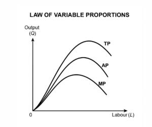
5. Law of Variable Proportions (Short Run)

Also known as the Law of Diminishing Returns.
It explains the effect of varying one input while keeping others fixed.

Statement

When additional units of a variable factor (e.g., labour) are applied to a fixed factor (e.g., land or capital), total output initially increases at an increasing rate, then at a diminishing rate, and eventually may decline.

Three Stages of Production

Stage	Behaviour of Output	Economic Meaning
Stage I – Increasing Returns	TP and MP rise rapidly	Underutilization of fixed factor
Stage II – Diminishing Returns	TP rises at decreasing rate	Optimal production zone
Stage III – Negative Returns	TP declines; MP negative	Overcrowding of variable input

6. Isoquant Analysis (Long-Run Production)

Isoquant

An isoquant curve represents combinations of two inputs (labour and capital) yielding the same level of output.
It is analogous to an indifference curve in consumer theory.

Properties of Isoquants

Downward sloping: To maintain output, more of one input requires less of the other.
Convex to origin: Reflects diminishing Marginal Rate of Technical Substitution (MRTS).
Do not intersect: Each represents distinct output level.
Higher isoquants: Indicate higher output levels.

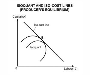
$M R T S_{L K} = - \frac{d K}{d L} = \frac{M P_{L}}{M P_{K}}$

Iso-Cost Line

Represents all input combinations a firm can buy for a given cost:

$C = w L + r K$

Where $w$ = wage rate and $r$ = rental rate of capital.
Slope = -w/r

Producer’s Equilibrium

Occurs where the isoquant is tangent to an iso-cost line:

$\frac{M P_{L}}{M P_{K}} = \frac{w}{r}$

This represents the least-cost combination of inputs.

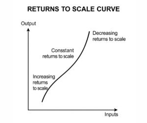
7. Returns to Scale (Long Run)

Examines how output responds to a proportionate change in all inputs.

Type	Description	Example
Increasing Returns to Scale (IRS)	Output increases more than proportionally.	Inputs ↑ 100% → Output ↑ > 100%
Constant Returns to Scale (CRS)	Output increases proportionally.	Inputs ↑ 100% → Output ↑ 100%
Decreasing Returns to Scale (DRS)	Output increases less than proportionally.	Inputs ↑ 100% → Output ↑ < 100%

Determinants of Returns to Scale

Indivisibility of inputs (e.g., machinery)
Specialization and division of labour
Managerial and technical efficiencies
Coordination challenges (for decreasing returns)

8. Theory of Costs

Cost refers to the expenditure incurred in producing goods and services.
It links production theory with financial decision-making.

Types of Costs

Cost Type	Definition	Example
Explicit (Actual)	Direct payments for inputs	Wages, rent, raw materials
Implicit (Imputed)	Value of self-owned resources	Owner’s labour, capital
Business Costs	Explicit + depreciation	Operational cost
Full Costs	Business + opportunity + normal profit	Economic cost
Out-of-Pocket	Cash payments	Wages, transport
Book Costs	Non-cash, accounting	Depreciation
Fixed Costs (TFC)	Remain constant with output	Rent, salaries
Variable Costs (TVC)	Vary with output	Raw materials, wages

Cost Functions

$T C = T F C + T V C$ $A C = \frac{T C}{Q}$ $M C = T C (n) - T C (n - 1)$

Relationships:

When MC < AC → AC falls
When MC > AC → AC rises
MC intersects AC at its minimum point

9. Cost Curves

Short-Run Cost Curves

AFC decreases continuously.
AVC and ATC are U-shaped due to economies and diseconomies of scale.
MC cuts both AVC and ATC at their minimum points.

Long-Run Cost Curves

All costs are variable.
LAC is the envelope of SRACs.
Traditionally U-shaped: reflects economies → constant returns → diseconomies of scale.

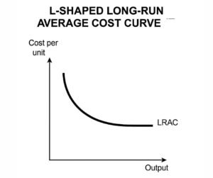
Modern (L-Shaped) Long-Run Cost Curve

Empirical evidence shows costs flatten out at high output.
Due to:
- Reserve capacity of plants
- Learning curve and technical improvement
- Economies persisting at large scale

10. Economies and Diseconomies of Scale

Economies	Diseconomies
Internal: technical, managerial, marketing, financial, risk spreading	Managerial inefficiency, coordination failure, communication delays
External: industry growth, localization, shared infrastructure	Resource scarcity, input price rise

11. Relationship Between Production and Cost

$M C = \frac{w}{M P_{L}}$

As Marginal Product rises → Marginal Cost falls.
When MP falls → MC rises.
Thus, productivity curves and cost curves are mirror images.

12. Private and Social Costs

Type	Meaning
Private Cost	Costs borne by the firm itself.
Social Cost	Private + external costs (e.g., pollution, congestion).

13. Key Definitions

Term	Definition
Isoquant	Curve showing input combinations yielding same output
MRTS	Rate of technical substitution between inputs
Fixed Cost	Cost that does not vary with output in short run
Marginal Cost	Cost of producing one additional unit
Economies of Scale	Cost advantages from larger scale
Social Cost	Total cost to society (private + external)

14. Important Graphs

1️⃣ Law of Variable Proportions
2️⃣ Isoquant–Iso-Cost Tangency (Producer’s Equilibrium)
3️⃣ Returns to Scale Curve
4️⃣ L-shaped Long-Run Average Cost Curve

(Refer to the attached academic diagrams page for illustration.)

15. Summary Table for UGC NET

Concept	Focus	Key Relation
Short-Run Law	Variable proportions	TP, MP, AP behaviour
Long-Run Law	Returns to scale	IRS, CRS, DRS
Isoquant Analysis	Producer equilibrium	$M P_{L} / M P_{K} = w / r$
Cost Analysis	U and L-shaped curves	MC–AC interaction
Scale Effects	Economies vs. Diseconomies	Internal & External

October 31, 2025

UGC NET Economics Unit-1 Theory of Consumer Behaviour MCQs-2

1.

In the indifference curve approach, consumer equilibrium is achieved when:
A) $M U_{x} / P_{x} = M U_{y} / P_{y}$
B) $M R S_{x y} = P_{x} / P_{y}$
C) $M R S_{x y} = M U_{x} / M U_{y}$
D) $P_{x} / P_{y} = M U_{y} / M U_{x}$
Answer: B

2.

Which of the following assumptions is not necessary for the ordinal utility approach?
A) Rational behaviour
B) Measurability of utility
C) Diminishing MRS
D) Transitivity of preferences
Answer: B

3.

The shape of an indifference curve showing perfect complements will be:
A) Downward-sloping straight line
B) Convex to the origin
C) L-shaped
D) Upward-sloping
Answer: C

4.

If a consumer’s income and all prices double, the budget line will:
A) Shift outward parallelly
B) Rotate about the origin
C) Remain unchanged
D) Become flatter
Answer: C

5.

The Law of Diminishing Marginal Utility forms the basis of:
A) Law of Demand
B) Law of Supply
C) Theory of Factor Pricing
D) Indifference Curve Analysis
Answer: A

6.

In Revealed Preference Theory, if a consumer chooses bundle A over B when both are affordable, it implies:
A) A is less preferred than B
B) A and B are equally preferred
C) A is revealed preferred to B
D) Prices are identical
Answer: C

7.

The slope of the budget line is equal to:
A) $- P_{x} / P_{y}$
B) $- P_{y} / P_{x}$
C) $M U_{x} / M U_{y}$
D) $M R S_{x y}$
Answer: A

8.

The indifference curve is convex to the origin because of:
A) Increasing MRS
B) Constant MRS
C) Diminishing MRS
D) Negative utility
Answer: C

9.

A straight-line indifference curve indicates:
A) Perfect substitutes
B) Perfect complements
C) No relation between goods
D) Inferior goods
Answer: A

10.

If MRS diminishes at a decreasing rate, indifference curves will be:
A) Linear
B) Steeper than normal
C) More convex
D) Less convex
Answer: D

11.

Consumer Surplus is the:
A) Difference between total utility and total expenditure
B) Difference between marginal utility and price
C) Ratio of utility to price
D) Product of utility and price
Answer: A

12.

Who first introduced the concept of Consumer Surplus?
A) J.R. Hicks
B) Alfred Marshall
C) Vilfredo Pareto
D) Paul Samuelson
Answer: B

13.

In the Hicksian method, Consumer Surplus is measured through:
A) Marginal Utility
B) Compensating and Equivalent Variations
C) Money Income
D) Revealed Preferences
Answer: B

14.

According to Samuelson’s Revealed Preference Theory, the Law of Demand can be derived without:
A) Indifference curves
B) Utility measurement
C) Budget constraints
D) Price ratios
Answer: B

15.

The tangency point between the budget line and indifference curve represents:
A) Minimum satisfaction
B) Maximum satisfaction
C) Equal satisfaction
D) Minimum expenditure
Answer: B

16.

If income increases and the prices of both goods remain constant, the budget line:
A) Shifts outward parallelly
B) Shifts inward parallelly
C) Rotates clockwise
D) Becomes vertical
Answer: A

17.

When the consumer’s equilibrium shifts due to a fall in price of good X, it is an example of:
A) Income effect only
B) Substitution effect only
C) Both income and substitution effects
D) Price effect
Answer: D

18.

The slope of the indifference curve measures:
A) Marginal Utility
B) Marginal Rate of Substitution
C) Price Ratio
D) Total Utility
Answer: B

19.

The Law of Equi-Marginal Utility states that a consumer allocates his expenditure such that:
A) $M U_{x} = M U_{y}$
B) $M U_{x} / P_{x} = M U_{y} / P_{y}$
C) $M U_{x} / M U_{y} = P_{x} / P_{y}$
D) $M U_{x} = P_{y}$
Answer: B

20.

Which of the following statements is true about a Giffen good?
A) Income effect is positive and greater than substitution effect
B) Substitution effect dominates income effect
C) Price effect is negative
D) Income effect and substitution effect are equal
Answer: A

21.

The Slutsky Equation decomposes the price effect into:
A) Income and substitution effects
B) Income and price effects
C) Price and demand effects
D) Substitution and cross-price effects
Answer: A

22.

A consumer’s equilibrium can also be expressed as:
A) $M U_{x} / P_{x} = M U_{y} / P_{y} = M U_{m}$
B) $M U_{x} / M U_{y} = P_{y} / P_{x}$
C) $M R S_{x y} = P_{x} / P_{y}$
D) All of the above
Answer: D

23.

If two indifference curves intersect, it violates:
A) Non-satiation
B) Rationality
C) Consistency and transitivity
D) Convexity
Answer: C

24.

The Ordinal Utility Theory was introduced by:
A) Alfred Marshall
B) Vilfredo Pareto
C) Lionel Robbins
D) Adam Smith
Answer: B

25.

The Revealed Preference Theory improves on Indifference Curve Analysis by:
A) Using real-life behaviour instead of assumptions
B) Measuring utility in numbers
C) Ignoring rationality
D) Using only one good
Answer: A

26.

The indifference curve approach was popularized through the work of:
A) Hicks and Allen
B) Pareto and Marshall
C) Robbins and Pigou
D) Keynes and Fisher
Answer: A

27.

A horizontal budget line implies that:
A) The price of good Y is zero
B) The price of good X is zero
C) The consumer has zero income
D) The goods are perfect complements
Answer: B

28.

If both income and the price of X double while the price of Y remains constant, the budget line will:
A) Shift outward
B) Shift inward
C) Rotate about the Y-axis
D) Remain unchanged
Answer: C

29.

In consumer theory, the substitution effect isolates:
A) Change in quantity demanded due to change in real income
B) Change due to change in relative prices
C) Change in utility level
D) Total price effect
Answer: B

30.

Under the Revealed Preference Hypothesis, preferences are assumed to be:
A) Random and inconsistent
B) Transitive, consistent, and rational
C) Constant but non-transitive
D) Dependent on income only
Answer: B

October 30, 2025
UGC NET Economics Unit-1 Theory of Consumer Behaviour MCQs-1

1.

The Indifference Curve technique assumes:
A) Utility is measurable in cardinal numbers.
B) Consumer behaviour is inconsistent.
C) Utility is comparable only in order of preference.
D) Marginal utility of money is diminishing.
Answer: C

2.

According to the Ordinal Utility approach, consumer equilibrium is obtained when:
A) The consumer attains maximum utility subject to income constraint.
B) Marginal utilities of goods are equal.
C) Price of one good equals its marginal utility.
D) Income equals total expenditure.
Answer: A

3.

Which of the following is not an assumption of the Indifference Curve analysis?
A) Rationality of the consumer
B) Constant income
C) Interdependence of utilities
D) Transitivity of preferences
Answer: C

4.

The Law of Equi-Marginal Utility can be expressed as:
A) $M U_{x} = M U_{y} = M U_{z}$
B) $M U_{x} / P_{x} = M U_{y} / P_{y} = M U_{z} / P_{z}$
C) $M U_{x} \times P_{x} = M U_{y} \times P_{y}$
D) $M U_{x} / M U_{y} = P_{x} / P_{y}$
Answer: B

5.

The slope of the Indifference Curve equals:
A) Marginal Rate of Substitution
B) Ratio of total utilities
C) Price ratio of goods
D) Marginal utilities of income
Answer: A

6.

If the price of good X falls and all else remains constant, the new equilibrium point will:
A) Move upward along the indifference map
B) Move downward along the same curve
C) Shift to a higher indifference curve
D) Remain unchanged
Answer: C

7.

Under Revealed Preference theory, a consumer reveals preference for bundle A over B when:
A) Bundle A is cheaper than B.
B) Both bundles yield equal utility.
C) A is chosen even when B was affordable.
D) Prices of goods remain constant.
Answer: C

8.

The Diminishing Marginal Rate of Substitution implies that:
A) Indifference curves are convex to the origin.
B) Indifference curves are straight lines.
C) Consumer preferences are inconsistent.
D) Goods are perfect complements.
Answer: A

9.

Which of the following combinations depicts consumer equilibrium under the Ordinal Utility approach?
A) $M R S_{x y} = M U_{x} / M U_{y}$
B) $M R S_{x y} = P_{x} / P_{y}$
C) $M U_{x} / P_{x} = M U_{y} / P_{y}$
D) $M U_{x} = M U_{y} = 0$
Answer: B

10.

The substitution effect shows:
A) Change in consumption due to change in real income.
B) Change due to change in relative prices of goods.
C) Change in total utility.
D) Shift in budget line parallelly outward.
Answer: B

11.

When two goods are perfect substitutes, the indifference curves will be:
A) Concave to the origin.
B) Convex to the origin.
C) L-shaped.
D) Straight lines.
Answer: D

12.

In Marshall’s concept of Consumer Surplus, utility is:
A) Ordinal
B) Cardinal and measurable in money terms
C) Relative
D) Socially determined
Answer: B

13.

Hicksian measurement of consumer surplus is based on:
A) Compensating and Equivalent Variations.
B) Law of Diminishing Marginal Utility.
C) Demand function only.
D) Revealed preferences.
Answer: A

14.

In the Indifference Curve analysis, the consumer’s budget line shifts parallelly outward when:
A) Prices fall in the same proportion.
B) Income increases.
C) Prices rise in the same proportion.
D) Income decreases.
Answer: B

15.

The Revealed Preference approach assumes that consumer behaviour is:
A) Irrational but measurable.
B) Consistent and transitive.
C) Random and unpredictable.
D) Dependent only on income.
Answer: B

16.

The equilibrium between marginal utilities and prices in the Cardinal approach indicates:
A) Maximization of satisfaction.
B) Minimization of expenditure.
C) Constant total utility.
D) Equality of total utilities.
Answer: A

17.

Which one of the following correctly expresses consumer equilibrium in the Cardinal Utility approach?
A) $M U_{x} / M U_{y} = P_{x} / P_{y}$
B) $M U_{x} / P_{x} = M U_{y} / P_{y} = M U_{m}$
C) $M U_{x} = P_{x} = M U_{y} = P_{y}$
D) $M U_{x} + M U_{y} = M U_{m}$
Answer: B

18.

The Slutsky Equation divides the price effect into:
A) Income effect + Substitution effect
B) Price effect + Utility effect
C) Income effect + Wealth effect
D) Price effect + Demand effect
Answer: A

19.

If two indifference curves intersect, the assumption violated is:
A) Rationality
B) Transitivity of preferences
C) Diminishing MRS
D) Completeness of choice
Answer: B

20.

The Law of Demand under Revealed Preference Theory can be derived because:
A) Utility is measurable.
B) Consumers behave inconsistently.
C) Price-quantity relationship is observable.
D) Consumers’ income remains fixed.
Answer: C

21.

Under Cardinal Utility theory, the marginal utility of money is assumed to be:
A) Constant
B) Increasing
C) Decreasing
D) Negative
Answer: A

22.

A rightward rotation of the budget line around the Y-axis indicates:
A) Fall in price of good X.
B) Increase in price of good Y.
C) Rise in consumer income.
D) Fall in income.
Answer: A

23.

In case of Giffen goods:
A) Both income and substitution effects reinforce each other.
B) Negative income effect outweighs substitution effect.
C) Substitution effect dominates income effect.
D) Price effect is positive.
Answer: B

24.

Consumer equilibrium changes to a higher indifference curve when:
A) Income decreases.
B) Price of one good rises.
C) Income increases or price falls.
D) Budget line becomes steeper.
Answer: C

25.

The Indifference Map represents:
A) All combinations giving different levels of satisfaction.
B) Combinations yielding the same utility.
C) Price combinations of goods.
D) Income levels at equilibrium.
Answer: A

26.

An upward-sloping indifference curve would indicate:
A) Normal goods.
B) Inferior goods.
C) Giffen goods.
D) Both goods are ‘bads’.
Answer: D

27.

In consumer theory, the substitution effect is always:
A) Negative
B) Positive
C) Neutral
D) Equal to price effect
Answer: B

28.

If the income effect is zero, the good must be:
A) Normal
B) Inferior
C) Neutral
D) Giffen
Answer: C

29.

The convexity of indifference curves reflects:
A) Diminishing MRS
B) Increasing MRS
C) Constant MRS
D) Increasing marginal utility
Answer: A

30.

According to Hicks, the main advantage of the Ordinal approach over the Cardinal one is:
A) It does not require utility measurement.
B) It eliminates the need for demand theory.
C) It measures satisfaction in monetary terms.
D) It assumes increasing marginal utility.
Answer: A

October 30, 2025

UGC NET Economics Unit 1-Theory of Consumer Behaviour

1. Introduction

The Theory of Consumer Behaviour deals with how consumers allocate their limited income among various goods and services to maximize satisfaction (utility). It forms the foundation of microeconomic analysis and demand theory.

The central question it addresses is:

“Given income and prices, what combination of goods will a rational consumer choose to maximize satisfaction?”

2. Approaches to the Theory of Consumer Behaviour

A. Cardinal Utility Approach (Marshallian Approach)

Assumptions

Measurable Utility: Utility can be measured in cardinal numbers like 1, 2, 3… (Utils).
Rational Consumer: The consumer aims to maximize total utility.
Diminishing Marginal Utility: As more of a good is consumed, the additional utility derived from each extra unit declines.
Independent Utilities: The utility of one commodity is independent of others.
Constant Marginal Utility of Money: The marginal utility of money remains unchanged.

Law of Diminishing Marginal Utility (DMU)

“As more units of a good are consumed, the additional satisfaction from each successive unit decreases.”

Mathematically:

$M U_{x} = \frac{Δ T U}{Δ Q_{x}}$

where $M U_{x}$ = Marginal Utility of good X, $Δ T U$ = change in total utility, $Δ Q_{x}$ = change in quantity consumed.

Consumer’s Equilibrium under Cardinal Utility

A consumer attains equilibrium when:

$\frac{M U_{x}}{P_{x}} = \frac{M U_{y}}{P_{y}} = M U_{m}$

where $M U_{m}$ is the marginal utility of money.

B. Ordinal Utility Approach (Indifference Curve Analysis)

Key Contributors

Vilfredo Pareto (1906), further developed by Hicks and Allen (1934) in Value and Capital.

Core Concept

Utility cannot be measured; it can only be ranked (ordered). Consumers can indicate preferences between bundles, not the exact level of satisfaction.

Assumptions

Rationality: Consumer seeks to maximize satisfaction.
Ordinal Utility: Preferences can be ordered (A preferred to B, etc.).
Transitivity: If A > B and B > C, then A > C.
Non-satiation: More of a good gives higher satisfaction.
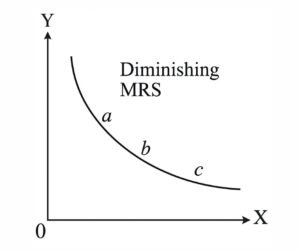
Diminishing Marginal Rate of Substitution (DMRS): As a consumer substitutes X for Y, the amount of Y he gives up for one more unit of X decreases.

3. Indifference Curve Analysis

Indifference Curve (IC)

An IC shows combinations of two goods that provide equal satisfaction to the consumer.
Thus, the consumer is indifferent among all combinations on the same IC.

Properties of Indifference Curves

Negatively Sloped: More of one good means less of the other to maintain same utility.
Convex to the Origin: Due to the law of diminishing MRS.
Non-Intersecting: Two ICs cannot cross each other.
Higher ICs Indicate Higher Utility: IC3 > IC2 > IC1.

Marginal Rate of Substitution (MRS)

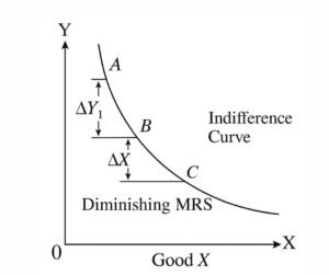
The rate at which the consumer is willing to give up Y for one more unit of X, keeping satisfaction constant.

$M R S_{x y} = - \frac{Δ Y}{Δ X}$

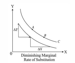
Diminishing MRS: As more of X is consumed, less of Y is sacrificed — hence IC is convex.

Budget Line

Represents all possible combinations of two goods that a consumer can buy with given income (M) and prices $P_{x}, P_{y}$ .

$P_{x} X + P_{y} Y = M$

Slope of the budget line: $- \frac{P_{x}}{P_{y}}$

Shifts:

Increase in income → Parallel outward shift.
Increase in price of one good → Rotation of line.

Consumer’s Equilibrium (Hicksian Equilibrium)

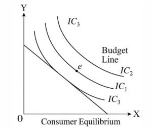
Occurs where Indifference Curve is tangent to the Budget Line:

$\frac{M U_{x}}{M U_{y}} = \frac{P_{x}}{P_{y}}$

At this point, MRS = Price Ratio. The consumer maximizes satisfaction given constraints.

4. Revealed Preference Theory (Samuelson, 1947)

This theory avoids the unobservable concept of utility. Instead, it relies on observed choices.

Assumptions

Rationality: Consumer prefers more to less.
Consistency: If A is preferred to B, B cannot be preferred to A.
Transitivity: If A > B and B > C, then A > C.
Stable Preferences: Preferences remain unchanged during analysis.

Axiom of Revealed Preference

If a consumer chooses bundle A over B when both are affordable, A is revealed preferred to B.

Implications

Law of Demand can be derived without measuring utility.
Indifference curves can be deduced from observed behaviour.

5. Theory of Consumer Surplus

Origin:

Introduced by A.J. Dupuit (1844) and later formalized by Alfred Marshall.

Meaning:

The difference between what a consumer is willing to pay and what he actually pays.

Mathematically:

$C S = T U - (P \times Q)$

Hicksian Measurement (Indifference Curve Method):

Hicks redefined consumer surplus in ordinal terms using indifference curves and budget constraints — a superior alternative to Marshall’s cardinal concept.

6. Criticisms and Limitations

Theory	Key Limitations
Cardinal Utility	Unrealistic measurability of utility; constant MU of money assumption.
Indifference Curve	Complex for more than two goods; assumes stable preferences.
Revealed Preference	Ignores psychological motives; assumes consistency.
Consumer Surplus	Cannot be precisely measured; not applicable to necessities.

7. Modern Developments in Consumer Behaviour

Behavioral Economics: Challenges the assumption of rationality (bounded rationality, heuristics, biases).
Expected Utility and Risk: Consumers make choices under uncertainty using probability-weighted utilities.
Intertemporal Choice: Examines consumption decisions over time (Fisher model).

8. Key Diagrams for UGC NET

Indifference Curve and Budget Line (Consumer Equilibrium)
Diminishing Marginal Rate of Substitution
Revealed Preference and Budget Constraint
Hicksian Consumer Surplus Measurement

9. Summary Points

The theory of consumer behaviour explains how consumers make choices under constraints.
Ordinal utility replaces cardinal measurement for realistic analysis.
Indifference curve analysis is central to modern microeconomics.
Revealed preference theory provides a scientific basis using observed choices.
Consumer surplus measures welfare from consumption.

10. Suggested Readings

Hicks, J.R. Value and Capital
Samuelson, P.A. Foundations of Economic Analysis
Dwivedi, D.N. Principles of Economics
Mankiw, G.N. Principles of Microeconomics
Koutsoyiannis, A. Modern Microeconomics

October 30, 2025

Tag: UGC NET Economics exam expected question

UGC NET Economics Unit 1-Theory of Production and Costs MCQs-1

1.

2.

3.

4.

5.

6.

7.

8.

9.

10.

11.

12.

13.

14.

15.

16.

17.

18.

19.

20.

21.

22.

23.

24.

25.

26.

27.

28.

29.

30.

UGC NET Economics Unit 1-Theory of Production and Costs

(Unit 1 – Microeconomics | UGC NET Economics)

1. Introduction

2. Classification of Inputs

3. Production Function

Features

4. Short-Run and Long-Run Production

5. Law of Variable Proportions (Short Run)

Statement

Three Stages of Production

6. Isoquant Analysis (Long-Run Production)

Isoquant

Properties of Isoquants

Iso-Cost Line

Producer’s Equilibrium

7. Returns to Scale (Long Run)

Determinants of Returns to Scale

8. Theory of Costs

Types of Costs

Cost Functions

9. Cost Curves

Short-Run Cost Curves

Long-Run Cost Curves

Modern (L-Shaped) Long-Run Cost Curve

10. Economies and Diseconomies of Scale

11. Relationship Between Production and Cost

12. Private and Social Costs

13. Key Definitions

14. Important Graphs

15. Summary Table for UGC NET

UGC NET Economics Unit-1 Theory of Consumer Behaviour MCQs-2

1.

2.

3.

4.

5.

6.

7.

8.

9.

10.

11.

12.

13.

14.

15.

16.

17.

$M U_{x} = \frac{Δ T U}{Δ Q_{x}}$

$\frac{M U_{x}}{P_{x}} = \frac{M U_{y}}{P_{y}} = M U_{m}$

$M R S_{x y} = - \frac{Δ Y}{Δ X}$

$P_{x} X + P_{y} Y = M$

$\frac{M U_{x}}{M U_{y}} = \frac{P_{x}}{P_{y}}$