Tag: UGC NET Economics study material

UGC NET Economics Unit 3 -Statistics and Econometrics

1. Probability Theory

Concept of Probability:

Probability measures the likelihood of an event occurring.
It always lies between 0 and 1.

$P (A) = \frac{Number of favourable outcomes}{Total number of outcomes}$

0 → Impossible event
1 → Certain event

Types of Probability:

Classical – based on equally likely outcomes (e.g., coin toss).
Empirical – based on past data (e.g., rainfall probability).
Subjective – based on personal judgment.

🔹 Important Concepts:

Independent Events: Occurrence of one doesn’t affect another.
Mutually Exclusive Events: Cannot occur simultaneously.
Conditional Probability:

$P (A ∣ B) = \frac{P (A \cap B)}{P (B)}$
Bayes’ Theorem: Used for revision of probabilities based on new information.

2. Probability Distributions

Discrete Distributions:

Binomial Distribution:

$P (x) = (\binom{n}{x}) p^{x} q^{n - x}$

Used for success-failure experiments.
Poisson Distribution:
Used when events are rare and independent (e.g., accidents).

$P (x) = \frac{e^{- λ} λ^{x}}{x!}$

🔹 Continuous Distribution:

Normal Distribution:
Bell-shaped curve; symmetric around mean.
Mean = Median = Mode.
Used in sampling, hypothesis testing, etc.

3. Moments and Central Limit Theorem

🔹 Moments:

Moments describe shape of a distribution.

1st moment → Mean
2nd moment → Variance
3rd moment → Skewness (asymmetry)
4th moment → Kurtosis (peakedness)

🔹 Central Limit Theorem (CLT):

As sample size increases, the sampling distribution of the sample mean approaches a normal distribution, regardless of population distribution.

💡 This theorem justifies the use of normal probability in statistics.

4. Descriptive Statistics

🔹 Measures of Central Tendency:

Mean (Average):

$\overset{ˉ}{X} = \frac{\sum X_{i}}{n}$
Median: Middle value when data arranged in order.
Mode: Most frequent value.

🔹 Measures of Dispersion:

Indicate how data values are spread around the mean.

Range
Variance
Standard Deviation
Coefficient of Variation (CV)

🔹 Correlation:

Shows relationship between two variables.
Karl Pearson’s coefficient:

$r = \frac{\sum (X - \overset{ˉ}{X}) (Y - \overset{ˉ}{Y})}{\sqrt{\sum (X - \overset{ˉ}{X})^{2} \sum (Y - \overset{ˉ}{Y})^{2}}}$

Values of r lie between -1 and +1.

🔹 Index Numbers:

Measure changes in price, quantity, or value over time.
Types:

Price Index (e.g., CPI, WPI)
Quantity Index
Value Index

Formulas:

Laspeyres Index: Base year weights
Paasche Index: Current year weights
Fisher’s Index: Geometric mean of the two (Ideal index)

5. Sampling Methods & Sampling Distribution

🔹 Sampling Methods:

Random Sampling – every unit has equal chance.
- Simple Random
- Stratified Random
- Systematic Sampling
- Cluster Sampling
Non-random Sampling – convenience or judgment-based.

🔹 Sampling Distribution:

Distribution of a statistic (like mean) from repeated random samples.
Used to estimate population parameters.

Standard Error (SE) = Standard deviation of a sampling distribution.

6. Statistical Inference and Hypothesis Testing

🔹 Estimation:

Point Estimate: single value (e.g., sample mean).
Interval Estimate: range of values (confidence interval).

🔹 Hypothesis Testing Steps:

State Null (H₀) and Alternative (H₁) hypotheses
Choose significance level (α)
Select appropriate test statistic (Z, t, χ², F)
Define rejection region
Calculate test statistic
Accept or reject H₀

🔹 Common Tests:

Z-test: Large samples (n > 30)
t-test: Small samples
χ²-test: Goodness of fit or independence
F-test: Compare two variances

7. Linear Regression Models

🔹 Simple Linear Regression:

$Y = α + β X + u$

where

Y = Dependent variable
X = Independent variable
u = Random error term

🔹 Properties of OLS (BLUE):

OLS estimators are Best Linear Unbiased Estimators when:

Linear in parameters
Expected value of error = 0
Homoscedasticity (constant variance)
No autocorrelation
No perfect multicollinearity
Errors are normally distributed

8. Identification Problem

Occurs in simultaneous equation systems when parameters cannot be uniquely estimated.

Identification Types:

Under-identified: Insufficient restrictions → No unique solution
Exactly identified: Just enough restrictions → Unique solution
Over-identified: More restrictions than needed → Multiple estimates

9. Simultaneous Equation Models

🔹 Recursive Models:

Equations arranged in sequence
No feedback
Can be solved by OLS

🔹 Non-Recursive Models:

Feedback present (mutual dependence)
Require Two-Stage Least Squares (2SLS) or Instrumental Variables (IV) for estimation.

10. Discrete Choice Models

Used when dependent variable is categorical (0/1, yes/no).

Types:

Logit Model – uses logistic function
Probit Model – uses cumulative normal distribution

Example: Probability of employment, adoption of technology, etc.

11. Time Series Analysis

Components of Time Series:

Trend (T): Long-term direction.
Seasonal (S): Regular pattern within a year.
Cyclical (C): Long-term up and down movements (business cycles).
Irregular (I): Random variations.

Models:

Additive Model: $Y = T + S + C + I$
Multiplicative Model: $Y = T \times S \times C \times I$

Stationarity:

A series is stationary when mean, variance, and covariance remain constant over time.

Autocorrelation:

Measures correlation between current and past values of a series.

AR, MA, ARMA, ARIMA Models:

Used for forecasting and economic time series modeling.

🧾 Quick Summary Table

Topic	Key Concept / Formula	Use / Importance
Probability	$P (A) = \frac{f}{n}$	Foundation of statistics
Normal Distribution	Bell-shaped curve	Basis for inference
CLT	Sample mean → normal	Enables hypothesis testing
Correlation	$r \in [- 1, + 1]$	Strength of relationship
Regression	$Y = a + b X$	Predictive analysis
BLUE	Best Linear Unbiased Estimator	Gauss-Markov theorem
Hypothesis Testing	Z, t, χ², F tests	Decision making
Identification	Unique estimation issue	Econometric modeling
Logit/Probit	Binary dependent variable	Discrete choice
Time Series	Trend, Seasonality, Cyclic	Forecasting

November 3, 2025

UGC NET Economics UNIT 1- MICROECONOMICS

(Summary Table)

(UGC NET & M.A. Economics Standard)

Topic	Core Concept / Definition	Key Formula / Relation / Diagram Reference	Major Economist(s)
1. Theory of Consumer Behaviour	Explains how a rational consumer allocates income to maximize satisfaction.	Utility Maximization: $M U_{X} / P_{X} = M U_{Y} / P_{Y}$ ; Budget Line: $P_{X} X + P_{Y} Y = M$	Alfred Marshall
2. Indifference Curve Analysis	Consumer equilibrium occurs at tangency of indifference curve and budget line.	$M R S_{X Y} = P_{X} / P_{Y}$ convex to origin	Hicks & Allen
3. Revealed Preference Theory	Preferences inferred from actual choices, not introspection.	Weak Axiom of Revealed Preference (WARP)	Paul Samuelson
4. Demand Function	Relationship between price and quantity demanded.	$Q_{d} = f (P, Y, T, P_{r}, E)$	Marshall
5. Elasticity of Demand	Measures responsiveness of demand to change in price, income, etc.	$E_{p} = \frac{Δ Q / Q}{Δ P / P}$	Marshall
6. Consumer Surplus	Extra satisfaction consumer derives over what he pays.	$C S = \int_{0}^{Q} D (Q) d Q - P Q$	Marshall
7. Cardinal Utility Analysis	Utility measurable in utils; based on diminishing marginal utility.	$M U = \frac{Δ T U}{Δ Q}$ ; $M U_{X} / P_{X} = M U_{Y} / P_{Y}$	Alfred Marshall
8. Ordinal Utility (Hicksian)	Consumer ranks bundles; equilibrium via indifference curves.	$M R S = P_{X} / P_{Y}$ ; Utility maximized where IC tangent to budget line	Hicks & Allen
9. Law of Demand	Price and demand inversely related, ceteris paribus.	$Q_{d} = a - b P$	Alfred Marshall
10. Giffen & Veblen Goods	Giffen goods show positive relation between P and Qd; Veblen goods due to status effect.	$\frac{d Q_{d}}{d P} > 0$	Sir Robert Giffen, Thorstein Veblen
11. Theory of Production	Shows relation between inputs and output.	$Q = f (L, K)$	J.B. Clark
12. Law of Variable Proportions	Short-run law: output increases at a decreasing rate beyond optimum input.	Three stages: Increasing, Diminishing, Negative returns	Marshall
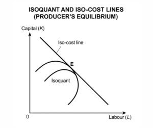
13. Isoquant & Isocost	Isoquant = combinations of inputs giving same output; Isocost = same cost.	Equilibrium: $M R T S_{L K} = \frac{w}{r}$	Hicks
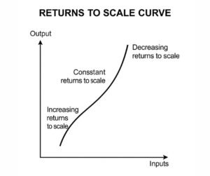
14. Returns to Scale	Long-run proportionate change in output due to change in all inputs.	CRS, IRS, DRS	Kaldor, Hicks
15. Cost Concepts	Relation between cost and output.	$T C = T F C + T V C$ ; $A C = T C / Q$ ; $M C = Δ T C / Δ Q$	Marshall
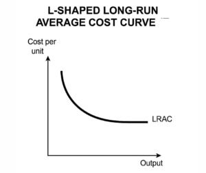
16. Short-run & Long-run Costs	In short run, some factors fixed; in long run, all variable.	LAC = Envelope of SAC curves	Marshall
17. Economies of Scale	Internal and external cost advantages due to size.	Decreasing LAC with scale	Alfred Marshall
18. Law of Supply	Positive relation between price and quantity supplied.	$Q_{s} = f (P)$	Marshall
19. Market Equilibrium	Achieved where demand = supply.	$Q_{d} = Q_{s}$ → $P^{}, Q^{}$	Walras
20. Perfect Competition	Many firms, homogeneous products, price takers, free entry/exit.	Profit max. at $M C = M R = P$	Cournot, Marshall
21. Monopoly	Single seller, price maker, downward-sloping demand curve.	$M R = M C$ ; $M R < P$ ; Lerner Index: $L = \frac{P - M C}{P}$	Joan Robinson
22. Monopolistic Competition	Product differentiation, many sellers, free entry.	$M R = M C$ in short run; Normal profit in long run	Chamberlin
23. Oligopoly	Few sellers, interdependence, strategic behavior.	Models: Cournot, Bertrand, Stackelberg, Kinked Demand	Cournot, Stackelberg, Sweezy
24. Duopoly	Two firms dominate the market.	Cournot: simultaneous output decisions; Stackelberg: leader–follower model	Cournot, Stackelberg
25. Price Discrimination	Same product sold at different prices without cost difference.	$M R_{1} = M R_{2} = M C$	Pigou
26. Game Theory	Analyzes strategic interdependence among rational players.	Payoff Matrix; Nash Equilibrium	John Nash
27. General Equilibrium Analysis	Simultaneous equilibrium in all markets.	Pareto Efficiency conditions: $M R S = M R T = M R T S$	Walras, Pareto
28. Pareto Optimality	No one can be made better off without making someone worse off.	Efficiency in exchange, production, and product mix	Vilfredo Pareto
29. Kaldor–Hicks Compensation Criterion	Welfare improves if gainers can compensate losers and still be better off.	Potential compensation principle	Kaldor & Hicks
30. Scitovsky Paradox	Logical inconsistency in Kaldor–Hicks test.	A→B and B→A both possible	T. Scitovsky
31. Social Welfare Function (SWF)	Social welfare depends on individual utilities.	$W = f (U_{1}, U_{2}, \dots, U_{n})$	Bergson & Samuelson
32. Utility Possibility Frontier (UPF)	Shows all efficient distributions of utilities.	Tangency of UPF & SWF → Maximum social welfare	Bergson, Hicks
33. Theory of Second Best	If one optimality condition fails, others may not hold.	Welfare can’t be improved by partial correction.	Lipsey & Lancaster
34. Externalities	Costs or benefits imposed on third parties without compensation.	Divergence between private & social cost/benefit	Pigou, Coase
35. Public Goods	Non-rival and non-excludable goods.	Free rider problem; Samuelson condition: $\sum M R S = M R T$	Paul Samuelson
36. Asymmetric Information	One party has more information than another.	Leads to adverse selection & moral hazard	Akerlof, Spence, Stiglitz
37. Adverse Selection	Hidden information before contract → low-quality participants.	Example: “Market for Lemons”	George Akerlof
38. Moral Hazard	Hidden actions after contract → risk-taking behavior.	Example: Insurance behavior	Stiglitz
39. Signaling & Screening	Tools to reduce info asymmetry.	Signaling (Spence); Screening (Stiglitz)	Spence, Stiglitz
40. Behavioral Economics	Incorporates psychology into rational choice models.	Prospect Theory; Bounded Rationality	Kahneman, Tversky, Simon

Quick Conceptual Recap

Theme	Core Question Answered	Key Equation / Idea
Consumer Behaviour	How individuals maximize satisfaction?	$M U_{X} / P_{X} = M U_{Y} / P_{Y}$
Producer Behaviour	How firms minimize cost or maximize output?	$M R T S_{L K} = w / r$
Market Structures	How firms interact and set prices?	$M C = M R$ ; varies by market type
Welfare Economics	How to judge social efficiency and welfare?	Pareto, Kaldor–Hicks, SWF
Information Economics	How imperfect info affects efficiency?	Adverse Selection, Moral Hazard

For Quick Exam Recall (UGC NET Keywords)

Consumer Equilibrium: $M R S = P_{X} / P_{Y}$
Producer Equilibrium: $M R T S = w / r$
Pareto Efficiency: $M R S = M R T = M R T S$
IS Curve (Goods Market): $Y = C + I + G$
LM Curve (Money Market): $M / P = L (Y, r)$
Phillips Curve: $π = π^{e} - β (u - u_{n})$
Rational Expectations: $Y = Y^{*} + α (π - π^{e})$

November 3, 2025

UGC NET Economics UNIT 2-MACROECONOMICS

1. NATIONAL INCOME: CONCEPTS AND MEASUREMENT

1.1 Meaning and Definition

National Income refers to the total value of all final goods and services produced within a country during a given period (usually a year).
It measures the economic performance and living standard of a nation.

$National Income = \sum (Value of Final Goods and Services)$

1.2 Basic Concepts

Concept	Definition	Symbol / Example
GDP (Gross Domestic Product)	Market value of all final goods & services produced within domestic territory.	$G D P = C + I + G + (X - M)$
GNP (Gross National Product)	GDP + Net factor income from abroad (NFIA).	$G N P = G D P + N F I A$
NNP (Net National Product)	GNP – Depreciation (capital consumption allowance).	$N N P = G N P - D e p r e c i a t i o n$
NNP at Factor Cost	NNP at Market Price – Indirect Taxes + Subsidies.	$N I = N N P_{f c}$
Personal Income (PI)	Income received by individuals before tax.	$P I = N I - (U n d i s t r i b u t e d P r o f i t s + C o r p o r a t e T a x e s$ $+ S o c i a l S e c u r i t y) + T r a n s f e r P a y m e n t$
Disposable Income (DI)	Income available for consumption & saving after tax.	$D I = P I - D i r e c t T a x e s$

1.3 Measurement Methods

Output (Production) Method:
- Measures total value added at each stage of production.
- Suitable for industrial economies.
$N I = \sum (V a l u e o f O u t p u t - I n t e r m e d i a t e C o n s u m p t i o n)$
Income Method:
- Sums all factor incomes: wages, rent, interest, profit.
$N I = W + R + I + P$
Expenditure Method:
- Sums all expenditures on final goods & services.
$N I = C + I + G + (X - M)$

1.4 Difficulties in Measurement

Double counting
Non-monetized sector
Illegal income and black money
Imputed values (e.g., owner-occupied housing)
Changing prices (inflation adjustment)

⚙️ 2. DETERMINATION OF OUTPUT AND EMPLOYMENT

2.1 Classical Theory of Employment (Say’s Law)

Core Assumptions:

Flexible prices and wages
Perfect competition
Full employment is the normal situation
Savings automatically equals investment via interest rate adjustment
Money is neutral (only medium of exchange)

Say’s Law of Markets:

“Supply creates its own demand.”

Hence, no general overproduction is possible. Unemployment is voluntary.

2.2 Keynesian Theory of Employment

Keynes (1936) rejected the classical view of automatic full employment.

Main propositions:

Employment depends on effective demand.
Effective Demand = Aggregate Demand (AD) = Aggregate Supply (AS).
Involuntary unemployment can persist due to deficiency of demand.

Aggregate Demand Function:

$A D = C + I$

Aggregate Supply Function:

$A S = f (N)$

Equilibrium Employment:
Occurs when

$A D = A S$ If

$A D < A S$ , unemployment arises.

2.3 Differences between Classical and Keynesian Models

Basis	Classical	Keynesian
Employment Level	Always full employment	May be less than full
Price & Wage	Flexible	Rigid in short run
Interest Role	Balances saving & investment	Investment depends on expectations
Government Role	Laissez-faire	Active fiscal policy
Money	Neutral	Non-neutral (affects output)

🏠 3. CONSUMPTION FUNCTION

3.1 Definition

Proposed by Keynes, the consumption function shows the relationship between consumption (C) and income (Y):

$C = f (Y)$

or $C = a + b Y$

where:

$a$ = autonomous consumption (independent of income)
$b$ = MPC = marginal propensity to consume

3.2 Marginal and Average Propensities

Measure	Formula	Meaning
MPC (Marginal Propensity to Consume)	$\frac{Δ C}{Δ Y}$	Change in consumption per unit change in income
APC (Average Propensity to Consume)	$\frac{C}{Y}$	Fraction of income spent on consumption

3.3 Psychological Law of Consumption (Keynes)

As income increases, consumption increases but by a smaller amount.

Thus: $0 < M P C < 1$

3.4 Determinants of Consumption

Income and wealth
Expectations and confidence
Distribution of income
Rate of interest
Fiscal policy
Credit availability

3.5 Theories of Consumption

Theory	Economist	Main Idea
Absolute Income Hypothesis	Keynes	Consumption depends on current income.
Relative Income Hypothesis	Duesenberry	Consumption depends on relative social status.
Permanent Income Hypothesis	Milton Friedman	Consumption depends on long-term (permanent) income.
Life Cycle Hypothesis	Modigliani	Individuals plan consumption over lifetime.

💸 4. INVESTMENT FUNCTION

4.1 Definition

Investment refers to expenditure on capital goods for future production.

$I = f (r, M E C, E x p e c t a t i o n s)$

4.2 Types of Investment

Induced Investment: Depends on income level.
Autonomous Investment: Independent of income.
Gross vs. Net Investment: Gross includes replacement; net = gross – depreciation.

4.3 Marginal Efficiency of Capital (MEC)

$M E C = \frac{E x p e c t e d A n n u a l R e t u r n s}{S u p p l y P r i c e o f C a p i t a l}$

Investment continues until

$M E C = R a t e o f I n t e r e s t$

4.4 Determinants of Investment

Rate of interest
Business expectations
Technological progress
Demand for products
Government policy
Availability of credit

🔁 5. MULTIPLIER AND ACCELERATOR

5.1 Multiplier Concept (Kahn & Keynes)

An initial increase in investment leads to a multiple increase in income and employment.

$k = \frac{1}{1 - M P C}$

$Δ Y = k \cdot Δ I$

Example:
If $M P C = 0.8$ $M$ , then

$k = 5$ ;
→ ₹1 crore investment increases income by ₹5 crore.

5.2 Accelerator Principle

Investment depends on the rate of change of output or income.

$I_{t} = v (Y_{t} - Y_{t - 1})$

where

$v$ = capital-output ratio.

The accelerator magnifies small changes in income into larger changes in investment.

5.3 Interaction of Multiplier and Accelerator (Super-Multiplier)

When both effects combine, economic fluctuations amplify — explaining business cycles.

💰 6. DEMAND FOR MONEY

6.1 Classical Theory (Quantity Theory of Money)

$M V = P T$

Money demand is only for transactions.
$V$

$V$ and $T$

$T$ are constant → money supply determines price level.

6.2 Keynesian Liquidity Preference Theory

Demand for money arises for:

Transactions motive (M₁)
Precautionary motive (M₂)
Speculative motive (M₃)

$L = L_{1} (Y) + L_{2} (r)$

At equilibrium: $M = L (Y, r)$

6.3 Friedman’s Modern Quantity Theory

$M_{d} = f (Y_{p}, r_{m}, r_{b}, r_{e}, π^{e})$

Money is treated as one of the assets; demand depends on permanent income and returns on other assets.

💵 7. SUPPLY OF MONEY

7.1 Definition

Money supply is the total stock of money (currency + deposits) available in the economy at a given time.

7.2 Measures of Money Supply (India – RBI Classification)

Measure	Components
M1 (Narrow Money)	Currency with public + Demand deposits + Other deposits with RBI
M2	M1 + Post office savings deposits
M3 (Broad Money)	M1 + Time deposits with banks
M4	M3 + Total post office deposits

7.3 High-Powered Money (Reserve Money)

$H = C + R$

where
C = currency held by public,
R = reserves of banks with the central bank.

7.4 Money Multiplier

$m = \frac{1}{C R + R R}$

Total money supply:

$M = m \times H$

🏦 8. IS–LM MODEL APPROACH

8.1 IS Curve (Investment–Saving Equilibrium)

Represents equilibrium in the goods market:

$Y = C (Y) + I (r) + G$

Downward-sloping — as interest rate ↓, investment ↑, output ↑.

8.2 LM Curve (Liquidity–Money Equilibrium)

Represents equilibrium in the money market:

$M / P = L (Y, r)$

Upward-sloping — as income ↑, demand for money ↑ → higher interest rate.

8.3 General Equilibrium

The intersection of IS and LM curves gives simultaneous equilibrium in both goods and money markets.

Situation	Description
IS right of LM	Excess demand → inflationary pressure
IS left of LM	Excess supply → unemployment

8.4 Fiscal and Monetary Policy in IS–LM

Fiscal Policy: Shifts IS curve (ΔG or ΔT).
Monetary Policy: Shifts LM curve (ΔM).
Crowding-out effect: Expansionary fiscal policy may raise interest rates, reducing private investment.

📈 9. INFLATION AND PHILLIPS CURVE

9.1 Inflation

Definition:
Sustained rise in general price level over time.

$I n f l a t i o n R a t e = \frac{P_{t} - P_{t - 1}}{P_{t - 1}} \times 100$

9.2 Types of Inflation

Type	Basis
Demand-pull	Excess aggregate demand
Cost-push	Increase in production costs
Creeping / Galloping / Hyper	Based on speed of inflation

9.3 Phillips Curve (A.W. Phillips, 1958)

Shows an inverse relationship between unemployment and inflation.

Short-run Phillips Curve (SRPC):
Inflation ↓ → Unemployment ↑.

Long-run Phillips Curve (LRPC):
Vertical at natural rate of unemployment (NAIRU).

Milton Friedman:
Argued no long-run trade-off — expectations adjust.

9.4 Expectations-Augmented Phillips Curve

$π = π^{e} - β (u - u_{n})$

where
π = actual inflation, πᵉ = expected inflation, u = unemployment, uₙ = natural rate.

🔄 10. BUSINESS CYCLES

10.1 Definition

Business cycles are recurrent fluctuations in economic activity (output, employment, income) around the long-term growth trend.

10.2 Phases

Expansion – rising output, investment, employment.
Peak – full employment, inflationary pressure.
Recession – decline in output and demand.
Trough – lowest point; high unemployment.
Recovery – renewed growth begins.

10.3 Theories of Business Cycles

Theory	Economist	Key Idea
Monetary Theory	Hawtrey	Fluctuations in credit and money supply
Keynesian Theory	Keynes, Hicks	Demand deficiency and multiplier–accelerator interaction
Schumpeterian Theory	Schumpeter	Innovations and technology cycles
Real Business Cycle Theory	Kydland & Prescott	Productivity shocks drive fluctuations

🏛️ 11. MONETARY AND FISCAL POLICY

11.1 Monetary Policy

Definition: Actions by the central bank to control money and credit to achieve economic stability.

Instruments:

Quantitative: CRR, SLR, Bank Rate, OMO, Repo.
Qualitative: Credit control, moral suasion, margin requirements.

Objectives:

Price stability
Employment
Economic growth
Exchange rate stability

11.2 Fiscal Policy

Definition: Government policy related to taxation, expenditure, and borrowing to influence economic activity.

Policy Type	Description
Expansionary	↑G, ↓T → boosts demand, reduces unemployment
Contractionary	↓G, ↑T → controls inflation

Fiscal Deficit:

$F i s c a l D e f i c i t = T o t a l E x p e n d i t u r e - (R e v e n u e R e c e i p t s + N o n - d e b t C a p i t a l R e c e i p t s)$

$F i sc a l De f i c i t = T o t a l E x p e n d i t u re - (R e v e n u e R ece i pt s + N o n - d e b t C a p i t a l R ece i pt s)$

Crowding Out:
Higher government spending may raise interest rates, reducing private investment.

12. RATIONAL EXPECTATIONS HYPOTHESIS (REH)

12.1 Concept

Proposed by John Muth (1961) and popularized by Robert Lucas (1972).

People form expectations about the future using all available information, including knowledge of government policies.

12.2 Implications

Markets are forward-looking and efficient.
Systematic policy changes (like predictable monetary expansion) have no real effect on output or employment — only on prices.
Economic agents do not make systematic errors.

$Y = Y^{*} + α (π - π^{e})$

→ If expectations are correct,

$π = π^{e}$ , hence $Y = Y^{*}$

12.3 Policy Ineffectiveness Proposition (Lucas)

Under rational expectations, anticipated fiscal and monetary policies are neutral; only unexpected policies can influence real variables.

12.4 Critique of Rational Expectations

Overly idealized: assumes perfect information processing.
Empirical evidence: short-run effects of policy still observed.
Bounded rationality: humans have cognitive limits (Herbert Simon).
Sticky prices and wages: prevent instant adjustment.

Summary Table — Unit 2: Macroeconomics

Topic	Core Concept / Definition	Key Formula / Relation	Major Economist(s)
National Income Accounting	Measures the total market value of all final goods and services produced in a year.	$Y = C + I + G + (X - M)$ ; $G N P = G D P + N F I A$	Simon Kuznets
Classical Employment Theory	Employment determined by real wage, Say’s Law — “Supply creates its own demand.”	$S = I$ via interest rate; $Q = f (L)$	J.B. Say, Ricardo, Pigou
Keynesian Employment Theory	Employment depends on effective demand (AD = AS).	$A D = C + I$ ; equilibrium when $A D = A S$	J.M. Keynes
Consumption Function	Consumption depends on income: $C = a + b Y$	$M P C = \frac{Δ C}{Δ Y}$ $A P C = \frac{C}{Y}$	J.M. Keynes
Theories of Consumption	Consumption behavior: absolute, relative, permanent, life-cycle.	–	Keynes, Duesenberry, Friedman, Modigliani
Investment Function	Investment depends on MEC (expected return) and rate of interest.	$M E C = \frac{R}{C}$ ; invest until $M E C = r$	J.M. Keynes
Multiplier Effect	Change in income due to change in investment.	$k = \frac{1}{1 - M P C}$ ; $Δ Y = k \cdot Δ I$	R.F. Kahn, J.M. Keynes
Accelerator Principle	Investment depends on change in income/output.	$I_{t} = v (Y_{t} - Y_{t - 1})$	J.M. Clark, Samuelson
Super-Multiplier	Combined effect of multiplier and accelerator.	$k^{'} = \frac{1}{1 - b - a v}$	Hicks, Samuelson
Demand for Money (Keynes)	Liquidity preference: transaction, precaution, speculative motives.	$L = L_{1} (Y) + L_{2} (r)$	J.M. Keynes
Modern Demand for Money	Money as an asset; depends on returns on other assets.	$M_{d} = f (Y_{p}, r_{m}, r_{b}, r_{e}, π^{e})$	Milton Friedman
Supply of Money	Total money stock available (currency + deposits).	$M = m \times H$ ; $m = \frac{1}{C R + R R}$	RBI, Friedman
IS–LM Model	Simultaneous equilibrium in goods (IS) and money (LM) markets.	IS: $Y = C + I + G$ : $M / P = L (Y, r)$	Hicks, Hansen
Inflation	Persistent rise in general price level.	$Inflation Rate = \frac{P_{t} - P_{t - 1}}{P_{t - 1}} \times 100$	Fisher, Keynes
Phillips Curve	Short-run trade-off between inflation and unemployment.	$π = π^{e} - β (u - u_{n})$	A.W. Phillips, Friedman
Business Cycles	Recurrent fluctuations in output and employment.	Phases: Expansion → Peak → Recession → Trough → Recovery	Schumpeter, Hicks
Monetary Policy	Central Bank control over money & credit to stabilize economy.	Instruments: CRR, SLR, Repo, OMO	RBI, Keynes, Friedman
Fiscal Policy	Government expenditure and taxation to manage demand.	$FD = T E - (R R + N D C R)$	Keynes
Crowding-Out Effect	Expansionary fiscal policy raises interest rates, reducing private investment.	$Δ I_{p} < 0$ $Δ$ when $i ↑$	Hicks, Hansen
Rational Expectations Hypothesis	People use all available information to form expectations.	$Y = Y^{*} + α (π - π^{e})$	J. Muth, R. Lucas
Policy Ineffectiveness (New Classical)	Anticipated policy changes have no real effect on output.	$π = π^{e} \Rightarrow Y = Y^{*}$	Lucas, Sargent
Critique of REH	Overestimates rationality; ignores sticky prices and bounded rationality.	–	Herbert Simon, Tobin

📚 SUGGESTED READINGS

Mankiw, N.G. – Macroeconomics
Dornbusch & Fischer – Macroeconomics
Ahuja, H.L. – Modern Economics
Froyen, R. – Macroeconomics: Theories and Policies
D.N. Dwivedi – Macroeconomics: Theory and Policy
Blanchard, O. – Macroeconomics
Snowdon & Vane – Modern Macroeconomics: Its Origins, Development and Current State

📚 SUGGESTED READINGS

Mankiw, N.G. – Macroeconomics
Dornbusch & Fischer – Macroeconomics
Ahuja, H.L. – Modern Economics
Froyen, R. – Macroeconomics: Theories and Policies
D.N. Dwivedi – Macroeconomics: Theory and Policy
Blanchard, O. – Macroeconomics
Snowdon & Vane – Modern Macroeconomics: Its Origins, Development and Current State

November 3, 2025

UGC NET Economics Unit 1-Asymmetric Information, Adverse Selection & Moral Hazard MCQs

Part A – Basic Concepts of Asymmetric Information (Q1–Q8)

1. Asymmetric information occurs when:

(A) All parties have the same information
(B) One party has more or better information than the other ✅
(C) Both parties have perfect knowledge
(D) Information is freely available to everyone

Explanation:
Asymmetric information means one side (buyer or seller) knows more about the transaction — e.g., seller knows product quality better.

2. The presence of asymmetric information may lead to:

(A) Perfect competition
(B) Market failure ✅
(C) Pareto efficiency
(D) Equilibrium at full employment

Explanation:
Unequal information distorts choices and contracts, often causing market inefficiency or failure.

3. Which of the following is NOT a consequence of asymmetric information?

(A) Adverse Selection
(B) Moral Hazard
(C) Market Signaling
(D) Price Discrimination ✅

Explanation:
Price discrimination relates to different pricing based on willingness to pay — not directly due to hidden information problems.

4. Information asymmetry violates which assumption of perfect competition?

(A) Free entry and exit
(B) Perfect knowledge ✅
(C) Homogeneous products
(D) Profit maximization

Explanation:
Perfect competition assumes all buyers and sellers are fully informed. Asymmetric information breaks this condition.

5. The study of markets with asymmetric information was developed prominently by:

(A) Keynes, Pigou, and Hicks
(B) Akerlof, Spence, and Stiglitz ✅
(C) Samuelson, Arrow, and Sen
(D) Marshall, Ricardo, and Walras

Explanation:
George Akerlof, Michael Spence, and Joseph Stiglitz shared the 2001 Nobel Prize for their work on information asymmetry.

6. An example of asymmetric information is:

(A) Buyer knowing car defects before seller
(B) Seller knowing car quality better than buyer ✅
(C) Both knowing all features
(D) Government fixing price ceiling

Explanation:
In Akerlof’s model, the seller knows whether the car is a “lemon” or a “peach,” while the buyer doesn’t — classic asymmetric information.

7. Which type of information problem occurs before a transaction?

(A) Moral Hazard
(B) Adverse Selection ✅
(C) Signaling
(D) Principal–Agent Problem

Explanation:
Adverse selection occurs before contracts are made — it’s caused by hidden information about risk or quality.

8. Which type of information problem occurs after a transaction?

(A) Adverse Selection
(B) Moral Hazard ✅
(C) Screening
(D) Asymmetric Signaling

Explanation:
Moral hazard arises after a deal is made — due to hidden actions that one party cannot monitor.

Part B – Adverse Selection (Q9–Q18)

9. Adverse selection means:

(A) Hidden information before contract ✅
(B) Hidden actions after contract
(C) Monitoring after contract
(D) Price discrimination by firm

Explanation:
Adverse selection occurs when one party withholds information before the transaction — leading to “bad” participants entering the market.

10. The concept of adverse selection was introduced by:

(A) Stiglitz
(B) Akerlof ✅
(C) Spence
(D) Arrow

Explanation:
George Akerlof’s paper “The Market for Lemons” (1970) analyzed how hidden information leads to market failure.

11. The “Market for Lemons” illustrates:

(A) Price discrimination
(B) Adverse selection ✅
(C) Monopoly pricing
(D) Externalities

Explanation:
In Akerlof’s example, used-car markets suffer because buyers can’t distinguish between good and bad cars.

12. In Akerlof’s lemons model, when buyers can’t distinguish product quality:

(A) Market price equals high-quality value
(B) Only high-quality goods are sold
(C) Average price causes good sellers to exit ✅
(D) Market efficiency increases

Explanation:
Good-quality sellers leave the market because the price doesn’t reflect their higher value → market collapse.

13. In insurance markets, adverse selection implies that:

(A) Low-risk individuals buy more insurance
(B) High-risk individuals are more likely to buy insurance ✅
(C) Everyone buys equal coverage
(D) Insurers can identify all risks

Explanation:
Since insurers can’t observe risk type, high-risk people self-select into buying more insurance.

14. In credit markets, adverse selection leads to:

(A) Lower interest rates
(B) Lenders offering less credit ✅
(C) Good borrowers dominating
(D) No impact on loan supply

Explanation:
Unable to distinguish good and bad borrowers, lenders raise interest rates or restrict credit, reducing loan supply.

15. Adverse selection is sometimes referred to as:

(A) Hidden Action Problem
(B) Hidden Information Problem ✅
(C) Hidden Incentive Problem
(D) Public Information Problem

Explanation:
It arises from hidden information that one side possesses prior to transaction.

16. In job markets, educational qualifications can serve as:

(A) Screening
(B) Signaling ✅
(C) Incentive constraint
(D) Hidden action

Explanation:
Michael Spence (1973) argued that education signals a worker’s ability to employers — reducing information asymmetry.

17. Screening refers to:

(A) Effort to hide information
(B) Method by which uninformed party extracts information ✅
(C) Promise of performance
(D) Concealing risk

Explanation:
Joseph Stiglitz’s concept — the uninformed side (e.g., insurer or employer) designs mechanisms to reveal the hidden characteristics.

18. Which of the following can reduce adverse selection?

(A) Signaling by informed parties ✅
(B) Reducing market competition
(C) Taxation
(D) Price control

Explanation:
Signaling (e.g., warranties, education, brand reputation) helps communicate private information and improve market outcomes.

Part C – Moral Hazard (Q19–Q27)

19. Moral hazard arises due to:

(A) Hidden information before contract
(B) Hidden actions after contract ✅
(C) Market competition
(D) Price rigidity

Explanation:
Moral hazard occurs when one party cannot observe the other’s actions after an agreement is made.

20. In insurance, moral hazard occurs when:

(A) Only high-risk people buy insurance
(B) Insured individuals behave more recklessly ✅
(C) Insurers raise premiums
(D) Information is perfect

Explanation:
After buying insurance, people may take less care since losses are covered — this is moral hazard.

21. Moral hazard occurs in the:

(A) Pre-contract stage
(B) Post-contract stage ✅
(C) Advertisement stage
(D) Screening stage

Explanation:
It arises after the agreement has been made and involves hidden or unobservable actions.

22. The principal–agent problem is an example of:

(A) Moral hazard ✅
(B) Adverse selection
(C) Price control
(D) Externality

Explanation:
When agents’ actions cannot be monitored, they may act against the principal’s interest — a moral hazard situation.

23. In moral hazard, incentives must be designed to ensure:

(A) Adverse selection
(B) Effort and performance alignment ✅
(C) Equal wages
(D) Higher interest rates

Explanation:
Contracts like bonuses, commissions, or performance pay align individual incentives with organizational goals.

24. Co-payment or deductibles in insurance help reduce:

(A) Adverse selection
(B) Moral hazard ✅
(C) Market signaling
(D) Free riding

Explanation:
By sharing part of the cost, insured persons remain cautious — mitigating risky behavior after insurance.

25. Monitoring and auditing are solutions to:

(A) Adverse selection
(B) Moral hazard ✅
(C) Inflationary gaps
(D) Monopoly power

Explanation:
Supervision ensures that agents act honestly and reduces hidden action problems.

26. The moral hazard problem can cause:

(A) Overuse of insured goods or services ✅
(B) Under-consumption of public goods
(C) Price rigidity
(D) Negative externality only

Explanation:
Because insured parties are shielded from costs, they tend to overconsume or behave less cautiously.

27. In the banking sector, moral hazard occurs when:

(A) Borrowers hide risk before loans
(B) Banks take excessive risks expecting government bailout ✅
(C) Banks charge high interest rates
(D) Depositors withdraw funds

Explanation:
If banks expect bailout (“too big to fail”), they may take higher risks — a moral hazard problem.

Part D – Comparative and Applied (Q28–Q30)

28. Difference between adverse selection and moral hazard is based on:

(A) Timing of the information problem ✅
(B) Type of market
(C) Nature of good
(D) Price elasticity

Explanation:
Adverse selection arises before contract (hidden info); moral hazard occurs after contract (hidden actions).

29. Principal–agent problem mainly deals with:

(A) Adverse selection before hiring
(B) Moral hazard after hiring ✅
(C) Information symmetry
(D) Price discrimination

Explanation:
Once the agent (employee) is hired, their effort can’t be perfectly monitored — a post-contract moral hazard.

30. Which policy measure can address both adverse selection and moral hazard?

(A) Reducing wages
(B) Improving transparency and information disclosure ✅
(C) Price ceilings
(D) Government subsidies

Explanation:
Improved information systems, reporting, and disclosure reduce both pre-contract (adverse selection) and post-contract (moral hazard) inefficiencies.

November 3, 2025

UGC NET Economics Unit 1-Asymmetric Information – Adverse Selection and Moral Hazard

1. Introduction

In traditional microeconomics, markets are assumed to have perfect information, meaning that buyers and sellers know everything relevant about the goods, prices, and market conditions.

However, in reality, information is imperfect and unevenly distributed — one party often knows more than the other.
This is known as Asymmetric Information, and it can cause market failures.

Definition:

Asymmetric Information occurs when one party in a transaction possesses more or better information than the other party.

Examples:

A used-car seller knows more about the car’s condition than the buyer.
A borrower knows more about their repayment ability than the lender.
An insured person knows more about their risk level than the insurance company.

Consequences of Asymmetric Information:

Market inefficiency
Adverse Selection
Moral Hazard
Principal–Agent Problem

2. Types of Asymmetric Information Problems

Type	When it occurs	Key Idea
Adverse Selection	Before a transaction	Hidden information about quality or risk leads to poor market outcomes.
Moral Hazard	After a transaction	Hidden actions after contract execution lead to opportunistic behavior.

3. Adverse Selection

Definition:

Adverse Selection refers to a situation where hidden information (before a transaction) causes high-risk or low-quality participants to dominate the market.

It happens before the deal is made because one side cannot distinguish between “good” and “bad” types.

Origin of Concept:

Developed by George Akerlof (1970) in his famous paper “The Market for Lemons”, which won him the Nobel Prize in Economics (2001).

Akerlof’s Example – “The Market for Lemons”

Used-car sellers know whether their cars are good (peaches) or bad (lemons).
Buyers can’t tell the difference and therefore offer an average price.
As a result:
- Sellers of good cars exit (since price is too low).
- Only “lemons” remain in the market.

👉 This leads to market failure — where only low-quality goods are traded, or the market may collapse completely.

3.1 Characteristics of Adverse Selection

Feature	Description
Timing	Occurs before transaction.
Type of information	Hidden information (quality or risk).
Effect	Drives out good participants; “bad drives out good.”
Market result	Market inefficiency or collapse.

3.2 Examples of Adverse Selection

Insurance Market:
- High-risk individuals are more likely to buy insurance.
- Insurer cannot distinguish between high- and low-risk customers.
- Leads to high premiums → low-risk people drop out.
Credit Market:
- Lenders cannot distinguish between good and bad borrowers.
- Charge a high interest rate → good borrowers avoid loans.
Labour Market:
- Employers cannot know workers’ productivity before hiring.
- High wages attract low-quality workers who intend to exploit firms.

3.3 Solutions to Adverse Selection

Solution	Explanation	Example
Signaling	The informed party provides credible information.	Education degrees as signals of ability (Spence, 1973).
Screening	The uninformed party designs mechanisms to reveal information.	Insurance company offering multiple policy options.
Warranties / Guarantees	Sellers assure buyers of product quality.	Warranty on used cars or electronics.
Reputation / Brand	Established firms build credibility over time.	Trusted brands reduce information asymmetry.

Key Economist Contributions:

George Akerlof (1970): “Market for Lemons” – Adverse Selection.
Michael Spence (1973): “Job Market Signaling.”
Joseph Stiglitz (1975): “Screening and Insurance.”
All three jointly received the 2001 Nobel Prize for their work on Asymmetric Information.

4. Moral Hazard

Definition:

Moral Hazard arises when one party changes their behavior after a contract is signed, because the other party cannot observe or verify their actions.

It occurs after the transaction, involving hidden actions rather than hidden information.

Example:

After getting insured, a person may take more risks, knowing the insurer bears the loss.
A manager may shirk after being hired because the employer cannot monitor them constantly.
A borrower may spend loan money irresponsibly once the loan is approved.

4.1 Characteristics of Moral Hazard

Feature	Description
Timing	Occurs after contract or transaction.
Type of Information	Hidden actions (effort, behavior).
Cause	Lack of monitoring or enforcement.
Effect	Inefficient outcomes, resource misuse, or higher costs.

4.2 Examples of Moral Hazard

Market	Example
Insurance Market	Insured individuals take more risks (e.g., drive carelessly).
Financial Market	Banks take risky investments expecting government bailouts.
Labour Market	Employees reduce effort after securing a job.
Corporate Sector	Managers pursue personal goals rather than shareholders’ interests.

4.3 Solutions to Moral Hazard

Solution	Explanation	Example
Incentive contracts	Align rewards with performance.	Bonus tied to productivity.
Monitoring & auditing	Observe and check actions.	Supervisors, audits in firms.
Deductibles / Co-payments	Share risk with insured to discourage recklessness.	Insurance deductibles.
Performance-based pay	Link pay to results.	Commissions, profit sharing.
Reputation mechanism	Repeat interactions encourage honesty.	Online seller ratings.

4.4 The Principal–Agent Problem

Principal: The one who delegates (e.g., employer, shareholder).
Agent: The one who acts on behalf of the principal (e.g., employee, manager).
When the agent’s actions are not observable, they may act in self-interest rather than in the principal’s interest.

➡️ This is a form of moral hazard due to asymmetric information after contract.

Examples:

Shareholders (principals) vs. managers (agents).
Government (principal) vs. contractors (agents).
Insurance company vs. insured person.

5. Comparison Between Adverse Selection and Moral Hazard

Feature	Adverse Selection	Moral Hazard
Timing	Before the transaction	After the transaction
Type of Problem	Hidden information	Hidden action
Key Concept	Wrong participants enter market	Participants change behavior after deal
Main Example	Buyer cannot judge product quality	Insured person becomes careless
Solution Methods	Signaling, screening, warranties	Incentive schemes, monitoring, deductibles

6. Policy Implications

Regulation and disclosure laws (e.g., mandatory product information).
Credit scoring systems to classify borrower risk.
Co-payments and deductibles in health insurance.
Performance-based compensation in management.
Government intervention to ensure transparency and information sharing.

7. Theoretical Contributions and Nobel Recognition

Economist	Contribution	Year
George Akerlof	Adverse selection (“Market for Lemons”)	1970
Michael Spence	Signaling in job markets	1973
Joseph Stiglitz	Screening and insurance behavior	1975
Joint Nobel Prize	For analysis of markets with asymmetric information	2001

8. Key Takeaways for UGC NET

Asymmetric Information → Unequal knowledge between parties.
Adverse Selection → Hidden information before contract → Market for lemons.
Moral Hazard → Hidden actions after contract → Risky behavior.
Principal–Agent Problem → A form of moral hazard.
Signaling and Screening → Tools to reduce information asymmetry.

9. Important Diagrams

(a) Adverse Selection – Market for Lemons

Demand curve: buyers’ expected price for average quality.
Supply curve: sellers’ willingness to sell.
Equilibrium shifts to low-quality goods only → market collapse.

(b) Moral Hazard – Principal–Agent Model

Principal offers contract: Pay = fixed + performance bonus.
Optimal contract balances risk sharing and incentive compatibility.

10. Summary Table

Concept	Timing	Hidden Factor	Main Example	Key Economist	Solution
Adverse Selection	Before contract	Hidden Information	Used-car market	Akerlof	Signaling, Screening
Moral Hazard	After contract	Hidden Action	Insurance market	Stiglitz	Incentive contracts, Monitoring
Principal–Agent Problem	After contract	Hidden Action	Employer–Employee	Jensen & Meckling	Performance pay, Supervision

📖 11. Suggested Readings

Akerlof, G. (1970) – The Market for Lemons: Quality Uncertainty and the Market Mechanism
Spence, M. (1973) – Job Market Signaling
Stiglitz, J. (1975) – Incentive Effects of Risk Sharing in Insurance
Hal R. Varian – Intermediate Microeconomics
Koutsoyiannis – Modern Microeconomics
D.N. Dwivedi – Microeconomics: Theory and Applications

November 3, 2025

UGC NET Economics Unit 1-Welfare Economics: Fundamental Theorems and Social Welfare Function

Part A – Basics of Welfare Economics (Q1–Q6)

1. The main objective of Welfare Economics is to:

(A) Study price determination
(B) Analyze economic growth
(C) Evaluate economic efficiency and social welfare ✅
(D) Maximize private profit

Explanation:
Welfare Economics studies how resource allocation affects collective welfare — combining efficiency and equity concerns.

2. Welfare Economics is concerned with:

(A) Positive analysis
(B) Normative analysis ✅
(C) Statistical analysis
(D) Descriptive economics

Explanation:
It makes value judgments about what is “good” or “bad” for society — thus, it is a normative branch of economics.

3. The two key aspects of Welfare Economics are:

(A) Growth and investment
(B) Efficiency and equity ✅
(C) Production and employment
(D) Savings and investment

Explanation:
Welfare economics deals with efficient use of resources (efficiency) and fair distribution (equity).

4. Which of the following is NOT a condition for Pareto Optimality?

(A) Efficiency in exchange
(B) Efficiency in production
(C) Efficiency in product mix
(D) Equal income distribution ✅

Explanation:
Pareto efficiency concerns resource use, not equality — even unequal allocations can be Pareto optimal.

5. In welfare economics, value judgments are:

(A) Avoided completely
(B) Necessary for social welfare comparisons ✅
(C) Not allowed in any case
(D) Based only on money

Explanation:
Value judgments are essential to define what society ought to prefer, especially in constructing a Social Welfare Function.

6. The welfare criterion that avoids interpersonal utility comparison is:

(A) Kaldor–Hicks
(B) Pareto criterion ✅
(C) Social welfare function
(D) Pigovian criterion

Explanation:
Pareto avoids comparing one person’s satisfaction with another — it only considers improvement without harm.

Part B – The Fundamental Theorems of Welfare Economics (Q7–Q17)

7. The First Fundamental Theorem of Welfare Economics states that:

(A) All efficient allocations are market equilibria
(B) Every competitive equilibrium is Pareto efficient ✅
(C) Monopoly ensures efficiency
(D) Redistribution increases welfare

Explanation:
Under perfect competition, equilibrium automatically leads to Pareto efficiency — that’s the first theorem.

8. The Second Fundamental Theorem states that:

(A) All Pareto efficient points are competitive equilibria after redistribution ✅
(B) Efficiency cannot coexist with equity
(C) Market equilibrium is always fair
(D) Government must fix prices

Explanation:
The second theorem shows that by redistributing initial endowments, any efficient point can be achieved through markets.

9. The First Welfare Theorem is based on the assumption of:

(A) Market imperfections
(B) Perfect competition ✅
(C) Monopoly power
(D) Price controls

Explanation:
It assumes perfectly competitive markets — with no externalities and perfect information.

10. The Second Welfare Theorem provides a theoretical justification for:

(A) Laissez-faire capitalism
(B) Redistributive policies ✅
(C) Fiscal deficit
(D) Monopoly regulation

Explanation:
It supports government redistribution to achieve desired equity, followed by free market functioning for efficiency.

11. According to the First Welfare Theorem:

(A) Markets always maximize social welfare
(B) Competitive equilibrium ensures Pareto efficiency ✅
(C) Monopoly markets are optimal
(D) Equity is automatically achieved

Explanation:
Competitive markets allocate resources efficiently, though they may not ensure fairness.

12. Pareto efficiency and market equilibrium coincide when:

(A) Market is imperfect
(B) Externalities exist
(C) Perfect competition prevails ✅
(D) Income is unequally distributed

Explanation:
Only under perfect competition does market equilibrium ensure Pareto optimality.

13. Which of the following is an assumption of both Welfare Theorems?

(A) Non-convex preferences
(B) Perfect competition ✅
(C) Increasing returns to scale
(D) Price rigidity

Explanation:
Both rely on perfect competition and convex preferences for efficiency.

14. The First Theorem of Welfare Economics links:

(A) Monopoly and fairness
(B) Competitive equilibrium and efficiency ✅
(C) Income distribution and taxation
(D) Growth and equity

Explanation:
It establishes that competitive market equilibrium results in a Pareto efficient allocation of resources.

15. The Second Theorem links:

(A) Redistribution and market equilibrium ✅
(B) Taxes and inefficiency
(C) Monopoly and price control
(D) Production and inflation

Explanation:
It demonstrates that redistribution of endowments can achieve any desired Pareto efficient point through markets.

16. The difference between the two theorems is that:

(A) The first is normative, the second positive
(B) The first is positive, the second normative ✅
(C) Both are purely descriptive
(D) Both are moral rules

Explanation:
The first describes (positive) how markets work; the second prescribes (normative) how redistribution can achieve fairness.

17. A limitation of the Second Welfare Theorem is that:

(A) It assumes lump-sum transfers are possible ✅
(B) It ignores competition
(C) It requires monopolies
(D) It forbids redistribution

Explanation:
The theorem assumes costless, distortion-free lump-sum transfers, which are unrealistic in practice.

Part C – The Social Welfare Function (SWF) (Q18–Q30)

18. The Social Welfare Function (SWF) was introduced by:

(A) Pareto
(B) Pigou
(C) Bergson ✅
(D) Hicks

Explanation:
Abram Bergson (1938) formulated the concept; Samuelson later refined it for modern welfare analysis.

19. The SWF expresses:

(A) Economic growth
(B) Aggregate income
(C) Society’s welfare as a function of individual utilities ✅
(D) Marginal productivity

Explanation:
It relates social welfare (W) to the utilities (U₁, U₂, …, Uₙ) of all individuals.

$W = f (U_{1}, U_{2}, U_{3}, \dots, U_{n})$

20. The SWF allows:

(A) No interpersonal utility comparison
(B) Explicit interpersonal utility comparisons ✅
(C) Only ordinal ranking
(D) Only money measurement

Explanation:
Unlike Pareto, SWF explicitly uses ethical or value judgments to compare utilities between individuals.

21. The SWF helps determine:

(A) The most efficient but unequal allocation
(B) The most preferred Pareto-efficient allocation ✅
(C) The richest individual’s welfare
(D) The producer’s surplus

Explanation:
Among many Pareto-efficient points, SWF selects the one that maximizes social welfare based on social values.

22. The Benthamite (Utilitarian) SWF maximizes:

(A) The welfare of the poorest
(B) The sum of individual utilities ✅
(C) The product of utilities
(D) The minimum utility

Explanation:
The utilitarian approach adds up all individuals’ utilities:

$W = U_{1} + U_{2} + \dots + U_{n}$

23. The Rawlsian (Max–Min) SWF focuses on:

(A) The richest group
(B) Average welfare
(C) Welfare of the worst-off individual ✅
(D) Total income

Explanation:
John Rawls emphasized justice and fairness — maximizing the welfare of the least advantaged person.

24. The Bernoulli–Nash (Multiplicative) SWF:

(A) Takes sum of utilities
(B) Takes product of utilities ✅
(C) Takes average utility
(D) Uses cardinal measures

Explanation:
It represents social welfare as a product:

$W = U_{1} \times U_{2} \times \dots \times U_{n}$

ensuring balance between equality and efficiency.

25. In the SWF diagram, the point of tangency between the Utility Possibility Frontier (UPF) and a Social Indifference Curve (SIC) shows:

(A) Economic growth
(B) Maximum social welfare ✅
(C) Minimum social welfare
(D) Perfect equality

Explanation:
The highest attainable social indifference curve tangent to the UPF identifies the welfare-maximizing allocation.

26. The SWF includes:

(A) Only individual utilities
(B) Both individual utilities and social value judgments ✅
(C) Only economic output
(D) None of the above

Explanation:
It combines measurable individual welfare and ethical judgments about their relative importance.

27. According to Arrow’s Impossibility Theorem:

(A) A perfect social choice function cannot exist ✅
(B) The SWF is always unique
(C) Pareto efficiency ensures fairness
(D) Redistribution reduces welfare

Explanation:
Kenneth Arrow proved that no voting system can aggregate individual preferences into a consistent social ranking satisfying all fairness conditions.

28. Which of the following violates Arrow’s fairness conditions?

(A) Dictatorship ✅
(B) Non-comparability
(C) Ordinality
(D) Efficiency

Explanation:
Dictatorship violates the principle of collective decision-making, as one person’s preferences dominate all others.

29. A limitation of the SWF is that:

(A) It ignores equality
(B) It requires interpersonal utility comparisons ✅
(C) It cannot handle multiple goods
(D) It is purely positive

Explanation:
The SWF depends on subjective judgments comparing utilities between individuals, which is ethically debatable.

30. The relationship among the three welfare tools is best summarized as:

(A) Welfare Theorems define efficiency; SWF adds equity ✅
(B) SWF ensures market equilibrium
(C) Welfare Theorems replace SWF
(D) SWF and Theorems are independent

Explanation:
The First and Second Welfare Theorems define efficient outcomes, while the SWF introduces social value judgments to choose among them.

November 3, 2025

UGC NET Economics Unit 1-Welfare Economics: Fundamental Theorems and Social Welfare Function

1. Introduction to Welfare Economics

Welfare Economics is a branch of microeconomics that studies how the allocation of resources affects social welfare — the collective well-being of society.

It tries to answer two essential questions:

Efficiency Question:
How can resources be allocated to achieve maximum total output or satisfaction?
(→ Efficiency analysis)
Equity Question:
How should resources and welfare be distributed among individuals?
(→ Distribution analysis)

Thus, welfare economics aims to design and evaluate economic policies that lead to the most efficient and just allocation of resources.

2. Objectives of Welfare Economics

To identify conditions for Pareto efficiency.
To analyze when market equilibrium is socially optimal.
To propose ways to improve social welfare through redistribution.
To develop a Social Welfare Function (SWF) to measure collective well-being.

3. Approaches to Welfare Economics

Approach	Basis	Key Economist	Focus
Cardinal Utility Approach	Utility measurable in absolute terms	Pigou	Total utility of society
Ordinal Utility / Pareto Criterion	Utility comparable in rank only	Pareto	Efficiency, not distribution
Compensation Principle	Potential compensation (Kaldor–Hicks)	Kaldor & Hicks	Practical welfare improvement
Social Welfare Function (SWF)	Value judgments included	Bergson & Samuelson	Ethical & social welfare analysis

4. The Two Fundamental Theorems of Welfare Economics

These theorems link competitive market equilibrium and Pareto efficiency — forming the foundation of modern welfare economics.

🧮 The First Fundamental Theorem of Welfare Economics

Statement:

“Every competitive equilibrium is Pareto efficient.”

Meaning:

Under certain ideal conditions, free markets automatically lead to an efficient allocation of resources without any external intervention.

If all agents act competitively and markets are complete, the equilibrium achieved is Pareto Optimal — no one can be made better off without hurting someone else.

Assumptions:

Perfect competition in all markets.
Rational consumers and firms (utility and profit maximization).
No externalities (production or consumption).
Perfect information (all agents fully informed).
Convex preferences and diminishing returns.
Complete markets for all goods and factors.

Implications:

Market mechanism ensures efficiency (allocative + productive).
Justifies laissez-faire policy (minimum government interference).
Explains why competitive markets are considered “efficient” systems.

Limitations:

Does not guarantee equity or fairness — an efficient allocation may still be highly unequal.
Assumes ideal market conditions rarely found in reality.
Ignores externalities, public goods, and asymmetric information.

⚖️ The Second Fundamental Theorem of Welfare Economics

Statement:

“Any Pareto efficient allocation can be achieved through competitive equilibrium, provided there is an appropriate redistribution of initial endowments.”

Meaning:

Equity and efficiency can be separated.
👉 The government can redistribute wealth or resources (to ensure fairness) and then allow free markets to reach an efficient outcome.

Assumptions:

Convex preferences and continuous utility functions.
Perfect competition in all markets.
Possibility of lump-sum redistribution (without distorting incentives).
No transaction costs or externalities.

Implications:

Efficiency and equity can be achieved simultaneously.
Government’s role: redistribute income, not control prices.
Establishes a normative policy framework — government adjusts endowments, markets ensure efficiency.

Graphical Explanation:

In an Edgeworth box, redistribution shifts the initial endowment point, leading to a new contract curveallocation.
Each new endowment point represents a different Pareto efficient outcome achievable through market exchange.

Limitations:

Lump-sum transfers are unrealistic (governments can’t perfectly redistribute).
Assumes perfect competition and no distortions.
Ignores transaction costs and political constraints.
Focuses only on efficiency — does not specify which allocation is “best” socially.

5. The Social Welfare Function (SWF)

Concept Origin:

Proposed by Abram Bergson (1938) and later refined by Paul A. Samuelson, the Social Welfare Function incorporates value judgments to evaluate alternative allocations.

Definition:

“The Social Welfare Function (SWF) represents the welfare of society as a function of the welfare (utility) of all individuals.”

Formally:

$W = f (U_{1}, U_{2}, U_{3}, \dots, U_{n})$

Where:

$W$ = Social welfare
$U_{i}$ = Utility of individual i
n = Number of individuals in society

Assumptions:

Society’s welfare depends on individual utilities.
Interpersonal comparison of utilities is allowed (value judgment).
Welfare is an increasing function of individual utilities.
Government or planner defines ethical weights for individuals’ utilities.

Interpretation:

Each point in the Utility Possibility Frontier (UPF) represents efficient allocations (Pareto Optimal).
The SWF identifies which point on the frontier maximizes overall social welfare.

Graphical Explanation:

Utility Possibility Frontier (UPF): All Pareto-efficient combinations of utilities of individuals A and B.
Social Indifference Curves (SICs): Show combinations of $U_{A}$ and $U_{B}$ giving equal social welfare.
The tangency between UPF and the highest SIC gives maximum social welfare.

Types of Social Welfare Functions

Type	Expression	Basis / Focus
Benthamite (Utilitarian)	$W = U_{1} + U_{2} + \dots + U_{n}$	Maximizes total utility (sum of happiness).
Rawlsian (Max–Min)	$W = \min (U_{1}, U_{2}, \dots, U_{n})$	Maximizes the welfare of the poorest.
Bernoulli–Nash	$W = U_{1} \times U_{2} \times \dots \times U_{n}$	Product form – balanced fairness and efficiency.
Egalitarian	$W = U_{1} = U_{2} = \dots = U_{n}$	Perfect equality.

Role of Value Judgments

Explicit value judgments are necessary to define social preferences (unlike Pareto).
The SWF is normative, reflecting society’s ethical priorities.
The choice of form (utilitarian, Rawlsian, etc.) determines the social goal — equality vs. efficiency trade-off.

Limitations of SWF

Interpersonal utility comparisons are subjective.
Determining weights for individuals’ utilities is difficult.
Arrow’s Impossibility Theorem (Kenneth Arrow, 1951) — no social choice rule can convert individual preferences into a consistent collective ranking satisfying fairness axioms.
Ignores non-utility aspects like freedom, justice, or rights (as Amartya Sen emphasized).

6. Relationship Between Welfare Theorems and SWF

First Theorem: Defines efficiency (Pareto optimality).
Second Theorem: Describes how to reach efficiency with equity through redistribution.
SWF: Selects the most desirable efficient allocation based on social value judgments.

Hence:

$Efficiency (Theorems) + Ethics (SWF) = Complete Welfare Economics$

7. Key Differences

Basis	First Theorem	Second Theorem	Social Welfare Function
Nature	Positive (descriptive)	Normative (redistributive)	Normative (ethical)
Focus	Efficiency of markets	Redistribution for equity	Overall social welfare
Role of Government	None	Redistribute endowments	Decide value weights
Utility Comparison	Not needed	Not needed	Needed
Main Concept	Pareto Efficiency	Feasible redistribution	Social choice with ethics

8. Importance in Policy Making

Justifies market mechanism for efficiency (Theorem I).
Justifies redistribution policies for equity (Theorem II).
Provides analytical foundation for welfare states.
SWF helps evaluate alternative policies on ethical and distributive grounds.

9. Key Terms Summary

Term	Meaning
Pareto Efficiency	No one can be better off without making another worse off.
Utility Possibility Frontier (UPF)	All possible Pareto-efficient utility combinations.
Social Indifference Curve (SIC)	All combinations of utilities giving same social welfare.
Bergson–Samuelson SWF	Function that ranks all possible social states based on ethical values.
Arrow’s Impossibility Theorem	No voting system can perfectly aggregate individual preferences into a social choice.

10. Summary

Concept	Essence	Policy Implication
First Welfare Theorem	Competitive equilibrium is Pareto efficient	Free markets yield efficiency
Second Welfare Theorem	Any Pareto efficient outcome can be achieved with redistribution	State can achieve equity + efficiency
SWF	Evaluates ethical desirability among Pareto efficient outcomes	Government sets welfare goals

📖 11. Suggested Readings

A.P. Lerner – Economics of Control
D.N. Dwivedi – Microeconomics: Theory and Applications
Paul A. Samuelson – Foundations of Economic Analysis
Koutsoyiannis – Modern Microeconomics
Amartya Sen – Collective Choice and Social Welfare
Hal R. Varian – Intermediate Microeconomics

November 3, 2025

UGC NET Economics Unit 1-Efficiency Criteria: Pareto-Optimality, Kaldor–Hicks & Wealth Maximization/MCQs

Part A – Pareto Efficiency (Q1–Q12)

1. A situation is Pareto optimal when:

(A) Everyone is equally well-off
(B) No one can be made better off without making someone worse off ✅
(C) Total utility is maximized
(D) Social welfare is at its peak

Explanation:
Pareto optimality means all mutual gains are exhausted — improving one person’s welfare necessarily harms another.

2. A Pareto improvement refers to:

(A) Everyone benefits equally
(B) At least one person gains and no one loses ✅
(C) Some gain and others lose
(D) Redistribution of income

Explanation:
A Pareto improvement makes at least one person better off while leaving others no worse off.

3. Pareto efficiency ensures:

(A) Fair income distribution
(B) Maximized total wealth
(C) Economic efficiency ✅
(D) Social justice

Explanation:
It is a test of efficiency, not equity — it says nothing about fairness or income equality.

4. Which economist first introduced the Pareto criterion?

(A) Alfred Marshall
(B) Vilfredo Pareto ✅
(C) A.C. Pigou
(D) Nicholas Kaldor

Explanation:
Italian economist Vilfredo Pareto (1906) developed the efficiency concept now called Pareto optimality.

5. Pareto optimality occurs when:

(A) $M R S_{A} = M R S_{B}$ ✅
(B) $M R T S_{A} = M R T S_{B}$
(C) $M R S \neq M R T$
(D) Marginal utilities are zero

Explanation:
In exchange efficiency, the marginal rates of substitution (MRS) between goods are equal for all individuals.

6. Efficiency in production under Pareto optimality requires:

(A) $M R T S_{L K}^{X} = M R T S_{L K}^{Y}$ ✅
(B) $M R S_{A} = M R S_{B}$
(C) $M R S = M R T$
(D) $M U_{X} = M U_{Y}$

Explanation:
Production efficiency demands equal MRTS (Marginal Rate of Technical Substitution) for all firms using the same factors.

7. Efficiency in product-mix requires:

(A) $M R S = M R T$ ✅
(B) $M R S_{A} = M R S_{B}$
(C) $M R T S_{X} = M R T S_{Y}$
(D) $M R S = M U$

Explanation:
For optimal product mix, the rate at which consumers are willing to substitute (MRS) equals the rate at which producers can transform goods (MRT).

8. Pareto Optimality implies:

(A) Equal income distribution
(B) Absence of waste ✅
(C) Maximum happiness
(D) Minimum cost

Explanation:
Pareto efficiency implies that no reallocation can increase someone’s welfare without reducing someone else’s — resources are fully utilized.

9. A limitation of Pareto Optimality is that:

(A) It allows interpersonal comparison of utilities
(B) It ignores distributional issues ✅
(C) It cannot show efficiency
(D) It depends on money income only

Explanation:
Pareto criterion is silent on how income or welfare is distributed — inequality can persist in a Pareto-efficient state.

10. In welfare economics, Pareto optimality is achieved when:

(A) Social welfare function is constant
(B) Exchange, production, and product-mix efficiencies exist ✅
(C) Government redistributes income
(D) Market prices are fixed

Explanation:
The three types of efficiency — exchange, production, and product mix — together define Pareto optimality.

11. Pareto criterion avoids:

(A) Value judgment
(B) Utility measurement
(C) Interpersonal comparison of utility ✅
(D) Price analysis

Explanation:
Pareto avoided comparing utilities across persons; his criterion is based on ordinal (non-comparable) preferences.

12. The Edgeworth box helps to explain:

(A) Business cycles
(B) Pareto efficiency in exchange ✅
(C) Monopoly power
(D) Externalities

Explanation:
The Edgeworth box graphically represents efficient allocations (Pareto optimal points) where indifference curves are tangent.

Part B – Kaldor–Hicks Compensation Criterion (Q13–Q22)

13. The Kaldor–Hicks criterion allows welfare improvement when:

(A) All individuals gain
(B) Gainers could compensate losers and still be better off ✅
(C) Actual compensation occurs
(D) Total income is redistributed

Explanation:
The test looks for potential compensation — gainers could compensate losers even if no payment is made.

14. The Kaldor–Hicks test is also known as:

(A) Actual compensation principle
(B) Potential compensation principle ✅
(C) Equity test
(D) Utility test

Explanation:
It measures potential welfare improvement, not actual transfers — hence, “potential compensation principle.”

15. The Kaldor–Hicks criterion is useful because:

(A) It includes ethical judgments
(B) It can evaluate policies that help some and harm others ✅
(C) It ensures equality
(D) It always benefits the poor

Explanation:
Unlike Pareto, it allows for trade-offs between winners and losers, making it practical for real-world policy evaluation.

16. Kaldor’s version emphasizes:

(A) Losers can bribe gainers
(B) Gainers can compensate losers ✅
(C) Everyone must gain
(D) Welfare remains constant

Explanation:
Kaldor stated that a change is desirable if gainers could compensate losers and still remain better off.

17. Hicks’s version of the criterion states that:

(A) Losers can bribe gainers not to change ✅
(B) Gainers always pay losers
(C) Equal compensation occurs
(D) Total income is constant

Explanation:
Hicks formulated the same idea oppositely — a change is desirable if losers cannot bribe gainers enough to prevent it.

18. The Kaldor–Hicks criterion is based on:

(A) Utility comparison
(B) Monetary evaluation of gains and losses ✅
(C) Equal utility
(D) Happiness index

Explanation:
It uses money value as a measure of welfare change, not direct utility.

19. The Kaldor–Hicks test resolves the main weakness of:

(A) Pareto criterion ✅
(B) Pigovian welfare theory
(C) Wealth maximization
(D) Utilitarianism

Explanation:
It overcomes Pareto’s limitation by allowing welfare analysis when some gain and others lose.

20. Which paradox questions the consistency of Kaldor–Hicks test?

(A) Edgeworth paradox
(B) Scitovsky paradox ✅
(C) Giffen paradox
(D) Bertrand paradox

Explanation:
Scitovsky showed that a move from A→B and then B→A can both satisfy the compensation test — hence inconsistency.

21. The compensation principle is most useful in:

(A) Monopoly theory
(B) Cost–benefit analysis ✅
(C) Labour economics
(D) Game theory

Explanation:
It provides a theoretical basis for cost–benefit analysis, where gains and losses are measured in monetary terms.

22. A criticism of Kaldor–Hicks is that:

(A) It’s too restrictive
(B) It ignores possibility of actual compensation ✅
(C) It always favors the poor
(D) It cannot be measured

Explanation:
The criterion tests for potential compensation, but in reality, losers are often not compensated.

Part C – Wealth Maximization (Q23–Q30)

23. The Wealth Maximization criterion was popularized by:

(A) Alfred Marshall
(B) Richard Posner ✅
(C) Nicholas Kaldor
(D) J.R. Hicks

Explanation:
Judge Richard A. Posner (Chicago School) promoted the idea that legal and economic efficiency is achieved through wealth maximization.

24. According to wealth maximization, efficiency is achieved when:

(A) Everyone’s utility is equal
(B) Total monetary value of resources is maximized ✅
(C) Income is equally distributed
(D) Market power is minimized

Explanation:
This approach focuses on maximizing total wealth, measured in monetary terms, not on individual satisfaction.

25. Wealth maximization is considered a:

(A) Moral criterion
(B) Monetary criterion ✅
(C) Utility-based test
(D) Egalitarian approach

Explanation:
It evaluates welfare in terms of monetary value of goods and resources rather than personal utility.

26. The Wealth Maximization criterion assumes:

(A) Market prices reflect individuals’ valuations ✅
(B) Utility is measurable
(C) Equality of income
(D) Perfect altruism

Explanation:
It is assumed that prices in competitive markets correctly measure how much people value goods and services.

27. The Wealth Maximization criterion is closely related to:

(A) Pareto criterion
(B) Kaldor–Hicks criterion ✅
(C) Marxian welfare theory
(D) Rawlsian justice theory

Explanation:
Wealth maximization is a monetized version of Kaldor–Hicks — focusing directly on aggregate market value.

28. In corporate economics, wealth maximization implies:

(A) Maximizing total sales
(B) Maximizing shareholders’ value ✅
(C) Equal distribution of profits
(D) Minimizing social costs

Explanation:
In business decision-making, the objective of wealth maximization means increasing the firm’s market value for shareholders.

29. A key limitation of wealth maximization is that it:

(A) Ignores distribution and equity ✅
(B) Lacks objectivity
(C) Cannot be quantified
(D) Requires welfare comparison

Explanation:
Since wealth maximization values outcomes by willingness to pay, it favors the rich, ignoring social fairness.

30. Wealth Maximization differs from Pareto optimality because it:

(A) Considers only efficiency
(B) Allows losers if total wealth rises ✅
(C) Requires all to gain
(D) Ignores money valuation

Explanation:
Pareto efficiency forbids making anyone worse off; wealth maximization permits some losses if aggregate wealth increases.

November 3, 2025

UGC NET Economics Unit 1-Efficiency Criteria — Pareto Optimality, Kaldor–Hicks, and Wealth Maximization

1. Introduction

Economic efficiency is a fundamental goal of welfare economics. It deals with how resources are allocated in society to maximize total satisfaction or welfare.

To judge whether an economic change or policy improves social welfare, economists have developed efficiency criteria— rules or tests to determine whether a given allocation or change increases overall economic efficiency.

The three major criteria are:

Pareto Optimality (Pareto Efficiency)
Kaldor–Hicks Compensation Principle
Wealth Maximization Criterion

2. Pareto Optimality (Vilfredo Pareto, 1906)

Definition

An allocation of resources is Pareto optimal (or Pareto efficient) when no one can be made better off without making someone else worse off.

In other words, all mutually beneficial gains from exchange have already been realized.

2.1 Pareto Improvement

A change from allocation A to B is a Pareto improvement if:

At least one person is better off, and
No one is worse off.

If no such improvement is possible, the allocation is Pareto Optimal.

2.2 Pareto Efficiency Conditions

A society achieves Pareto efficiency when three efficiency conditions are met:

Type of Efficiency	Condition	Explanation
(i) Exchange Efficiency	$M R S_{X Y}^{A} = M R S_{X Y}^{B}$	Marginal rates of substitution between goods are equal for all consumers.
(ii) Production Efficiency	$M R T S_{L K}^{X} = M R T S_{L K}^{Y}$	Marginal rates of technical substitution between factors are equal across all firms.
(iii) Product-Mix Efficiency	$M R S_{X Y} = M R T_{X Y}$	The rate at which consumers trade goods equals the rate at which producers can transform them.

When all three hold simultaneously, the economy is in general equilibrium and is Pareto optimal.

2.3 Graphical Representation

In an Edgeworth Box (Exchange), Pareto efficiency occurs at tangency points of the two consumers’ indifference curves — forming the Contract Curve.
In Production, it occurs where the isoquants of two firms are tangent (equal MRTS).
Combining both gives the Production Possibility Frontier (PPF), where efficiency requires $M R S = M R T$ .

2.4 Limitations of Pareto Criterion

No Interpersonal Comparison of Utility:
It cannot decide between policies that help one person and harm another.
Insensitive to Distribution:
A situation with extreme inequality can still be Pareto efficient.
Static Criterion:
It doesn’t account for long-term growth or dynamic welfare.
Unrealistic in Policy:
Real-world changes usually benefit some and hurt others — true Pareto improvements are rare.

3. Kaldor–Hicks Compensation Principle

Because Pareto efficiency was too restrictive, economists Nicholas Kaldor (1939) and John Hicks (1940) proposed a more practical test for welfare improvement.

3.1 The Kaldor–Hicks Criterion

A change or policy is considered welfare-improving if:

“The gainers from a policy could compensate the losers and still be better off — even if no actual compensation occurs.”

This is known as the Potential Pareto Improvement.

3.2 Example

Suppose a new project increases firm profits by ₹100 crore but reduces workers’ income by ₹40 crore.
→ Even if the firm could hypothetically compensate workers ₹40 crore and still gain ₹60 crore, the project passes the Kaldor–Hicks test.

3.3 Hicks’s Version

Hicks proposed the same idea from the loser’s point of view:

“A policy is desirable if the losers cannot bribe the gainers enough to stop the change.”

3.4 Diagrammatic Explanation

On a utility possibility frontier (UPF):

Each point represents combinations of utilities of two individuals (A and B).
Movement from point P to Q that makes A better off and B worse off is Kaldor-improving if A could compensate B to reach a higher potential welfare frontier.

3.5 Advantages of Kaldor–Hicks

Allows for trade-offs between gains and losses.
Practical for cost–benefit analysis and policy evaluation.
Focuses on potential improvements, not actual compensation.

3.6 Limitations

No guarantee of actual compensation: losers may remain worse off.
Distributional bias: may favor the rich if their monetary gains outweigh the poor’s losses.
Reversibility problem (Scitovsky Paradox):
- A move from A → B may satisfy Kaldor’s test,
- but a move back from B → A may also satisfy Hicks’s test,
  showing inconsistency.

4. Wealth Maximization Criterion (Harold Demsetz, Richard Posner)

The Wealth Maximization approach comes from the Chicago School of Law and Economics, particularly Richard Posner (1979).
It is often used in law, policy, and corporate economics as a decision criterion.

4.1 Definition

A policy, decision, or allocation is considered efficient if it maximizes the total monetary value of society’s wealth, irrespective of individual welfare distribution.

It focuses on aggregate wealth, not on utility or satisfaction.

4.2 Basic Principle

All goods and rights are valued by what people are willing to pay for them (market prices).
If resources are reallocated to higher-valued uses, total wealth increases, even if some individuals lose.

4.3 Relation to Kaldor–Hicks

Wealth maximization is essentially a monetized version of the Kaldor–Hicks principle.
It assumes market prices reflect individuals’ utilities and preferences.

4.4 Application

Used in:

Corporate decision-making — maximize shareholder wealth.
Legal analysis — efficient laws are those that maximize total wealth (Posner’s view).
Cost–Benefit Analysis — projects with the highest net monetary gain are preferred.

4.5 Advantages

Practical and measurable: uses monetary value as a common yardstick.
Objective: avoids subjective utility comparisons.
Decision-making simplicity: clear rule for economic policy and business evaluation.

4.6 Limitations

Neglects distribution and equity: benefits the rich more if they have higher “willingness to pay.”
Ignores non-market values: such as environment, justice, or ethics.
Assumes perfect markets and rational valuation, which are rarely true.

5. Comparative Overview

Criteria	Key Idea	Test for Welfare Improvement	Advantages	Limitations
Pareto Optimality	Efficiency without harming anyone	At least one better off, no one worse	Exact and morally appealing	Too restrictive, ignores equity
Kaldor–Hicks	Potential compensation principle	Gainers could compensate losers	Practical, used in policy	No actual compensation, may favor rich
Wealth Maximization	Maximize total monetary value	Higher total wealth = efficiency	Simple, objective	Ignores fairness and non-market values

6. Summary

Pareto Optimality: Ideal but impractical criterion for efficiency; no one can be hurt.
Kaldor–Hicks Efficiency: Practical, allows trade-offs; used in cost–benefit analysis.
Wealth Maximization: Simplifies efficiency into total monetary value; widely used in law and business, but ignores distribution.

Thus, these criteria form a progressive relaxation of constraints:

$Pareto (Strict) \Rightarrow Kaldor–Hicks (Flexible) \Rightarrow Wealth Maximization (Pragmatic)$

7. Key Terms

Term	Meaning
Pareto Improvement	A change that benefits someone without hurting anyone else.
Compensation Principle	Welfare improves if gainers can potentially compensate losers.
Scitovsky Paradox	Both forward and reverse moves may satisfy Kaldor–Hicks test.
Utility Possibility Frontier (UPF)	Curve showing all efficient utility combinations for two individuals.
Wealth Maximization	Economic criterion emphasizing total wealth increase, not fairness.

8. Important UGC NET Short Notes

First Welfare Theorem: Every competitive equilibrium is Pareto Efficient.
Second Welfare Theorem: Any Pareto Efficient allocation can be reached through redistribution of initial endowments.
Kaldor–Hicks Criterion = Potential Pareto Improvement.
Wealth Maximization is the operational form of Kaldor–Hicks efficiency used in Law and Economics.

📖 9. Suggested Readings

D.N. Dwivedi – Microeconomics: Theory and Applications
Koutsoyiannis – Modern Microeconomics
Hal R. Varian – Intermediate Microeconomics
A.K. Sen – Collective Choice and Social Welfare
Richard Posner – Economic Analysis of Law

November 3, 2025

UGC NET Economics Unit 1-General Equilibrium Analysis MCQs

Part A – Fundamentals of General Equilibrium (Q1–Q10)

1. The general equilibrium approach was first developed by:

(A) Alfred Marshall (B) Léon Walras ✅ (C) Vilfredo Pareto (D) Adam Smith

Explanation:
Léon Walras introduced the concept of general equilibrium in his 1874 book Elements of Pure Economics. He used simultaneous equations to show how all markets in an economy reach equilibrium together.

2. The partial equilibrium analysis assumes:

(A) Interdependence of all markets
(B) Simultaneous equilibrium of all markets
(C) Other things remain constant ✅
(D) Constant returns to scale

Explanation:
Partial equilibrium (Marshallian) isolates one market at a time, assuming ceteris paribus — all other factors such as incomes, prices of related goods, and tastes remain constant.

3. General Equilibrium analysis considers:

(A) One market in isolation
(B) All interrelated markets simultaneously ✅
(C) Only factor markets
(D) Only goods markets

Explanation:
General equilibrium recognizes interdependence among all markets (goods and factors) and determines prices and quantities in all of them together.

4. Equality of demand and supply in all markets simultaneously is known as:

(A) Microeconomic equilibrium
(B) General equilibrium ✅
(C) Partial equilibrium
(D) Market failure

Explanation:
General equilibrium occurs when demand equals supply in every market of an economy at the same time.

5. The Walrasian system uses which mathematical method?

(A) Differential equations
(B) Simultaneous equations ✅
(C) Regression analysis
(D) Integral calculus

Explanation:
Walras modeled markets as a system of simultaneous equations, where all prices and quantities are determined together.

6. In Walrasian analysis, “unknowns” represent:

(A) Quantities only
(B) Prices only
(C) Prices and quantities of all commodities and factors ✅
(D) Profits and wages only

Explanation:
The Walrasian model includes as many unknowns (prices and quantities) as independent equations for all goods and factors in the system.

7. Walras’ Law states that:

(A) The sum of excess demands across markets equals zero ✅
(B) Total supply always exceeds demand
(C) Only one market can be in equilibrium
(D) Demand always exceeds supply

Explanation:
Walras’ Law implies that if n-1 markets are in equilibrium, the nth market must also be in equilibrium — the sum of excess demands times prices is always zero.

8. If all but one market are in equilibrium, then according to Walras’ Law:

(A) No equilibrium exists
(B) The last market must also be in equilibrium ✅
(C) Prices will diverge
(D) Supply exceeds demand

Explanation:
Because total value of excess demand is zero, equilibrium in all but one market automatically ensures equilibrium in the remaining market.

9. The existence of a general equilibrium solution requires:

(A) More unknowns than equations
(B) Equal number of independent equations and unknowns ✅
(C) Fewer equations than unknowns
(D) No mathematical relationship

Explanation:
A basic mathematical requirement for solvability of the Walrasian system is equality between the number of independent equations and the number of unknown variables.

10. The Arrow–Debreu model proved:

(A) Instability of equilibrium
(B) Existence of general equilibrium ✅
(C) Monopoly equilibrium
(D) Disequilibrium in markets

Explanation:
Kenneth Arrow and Gérard Debreu (1954) gave a rigorous proof that, under convex preferences and continuous production functions, a general equilibrium always exists.

Part B – Existence, Uniqueness & Stability (Q11–Q20)

11. The existence of equilibrium depends on:

(A) Equality of equations and unknowns
(B) Convex preferences and diminishing returns ✅
(C) Constant costs
(D) Increasing returns

Explanation:
Arrow–Debreu showed that general equilibrium exists if preferences are convex and production exhibits constant or diminishing returns.

12. Uniqueness of equilibrium means:

(A) Multiple equilibria
(B) Only one set of prices clears all markets ✅
(C) No solution
(D) Negative prices

Explanation:
Uniqueness ensures a single consistent price–quantity combination that balances all markets; otherwise, multiple equilibria can arise.

13. A stable equilibrium is one where:

(A) Disturbances push the system away
(B) The system returns to equilibrium after disturbance ✅
(C) Output stays fixed
(D) Price never changes

Explanation:
Stability means that self-correcting forces (supply and demand) restore equilibrium when disturbed — essential for market resilience.

14. The Cobweb theorem illustrates:

(A) Market failure
(B) Dynamic stability and instability ✅
(C) Monopoly behavior
(D) Welfare loss

Explanation:
The Cobweb theorem analyzes oscillations in price and output over time due to lagged supply responses, showing conditions for stability.

15. In the Cobweb model, if demand is steeper than supply (|dP/dQ| < |sP/dQ|):

(A) The system is stable ✅
(B) The system diverges
(C) It is neutral
(D) Unattainable equilibrium

Explanation:
When the demand curve is flatter (less steep) than the supply curve, price and quantity adjustments converge toward equilibrium.

16. If slopes of demand and supply are equal in Cobweb model:

(A) Stable
(B) Neutral oscillations (undamped) ✅
(C) Explosive
(D) Divergent

Explanation:
Equal slopes cause constant oscillations around equilibrium — neither converging nor diverging — known as neutral or undamped cycles.

17. Multiple equilibria occur when:

(A) Demand curve is backward bending ✅
(B) Supply curve is linear
(C) Cost curve is flat
(D) Production is constant

Explanation:
Backward-bending demand (as for inferior goods) can intersect supply more than once, yielding multiple equilibrium points.

18. The Arrow–Debreu model assumes:

(A) Convex preferences, no externalities ✅
(B) Increasing returns
(C) Non-convex utility
(D) Monopoly

Explanation:
For equilibrium to exist, Arrow–Debreu required convex preferences, continuous functions, and absence of externalities or joint production.

19. A unique and stable equilibrium exists under:

(A) Perfect competition and diminishing returns ✅
(B) Monopoly power
(C) Increasing returns
(D) Oligopoly

Explanation:
Perfect competition with diminishing returns ensures no incentive for divergence — yielding stable and unique equilibrium.

20. The automatic adjustment process in general equilibrium works best under:

(A) Government price control
(B) Perfect competition ✅
(C) Monopoly
(D) Price rigidity

Explanation:
Only under perfect competition can prices freely adjust through supply and demand, restoring equilibrium automatically.

Part C – Pareto Efficiency & Welfare (Q21–Q30)

21. Pareto Efficiency occurs when:

(A) Total utility is maximized
(B) No one can be made better off without making someone worse off ✅
(C) Equal income distribution
(D) Government maximizes welfare

Explanation:
A Pareto efficient allocation means all possible mutual gains from trade have been exhausted.

22. Efficiency in Exchange requires:

(A) MRTS equality
(B) MRT equality
(C) Equal MRS between individuals ✅
(D) Equal incomes

Explanation:
Exchange efficiency holds when the Marginal Rate of Substitution (MRS) between goods is the same for all consumers.

23. Efficiency in Production requires:

(A) MRTS_X = MRTS_Y ✅
(B) MRT = MRS
(C) MU_X = MU_Y
(D) Equal factor prices only

Explanation:
Production efficiency occurs when the Marginal Rate of Technical Substitution (MRTS) between factors is equal across firms.

24. Efficiency in Product Mix requires:

(A) MRS = MRT ✅
(B) MRTS_X = MRTS_Y
(C) MC = MR
(D) Equal profits

Explanation:
For optimal output mix, the Marginal Rate of Transformation (MRT) in production equals consumers’ MRS in consumption.

25. Pareto Efficiency is achieved when:

(A) Exchange, production, and product-mix efficiencies all hold ✅
(B) Only exchange is efficient
(C) Factor allocation is fixed
(D) Price = average cost

Explanation:
All three efficiencies (exchange, production, and product mix) together define a Pareto optimal general equilibrium.

26. First Welfare Theorem states:

(A) Every Pareto efficient allocation is competitive
(B) Every competitive equilibrium is Pareto efficient ✅
(C) Equity and efficiency coincide
(D) Monopoly leads to efficiency

Explanation:
Under perfect competition and no externalities, market equilibrium automatically leads to Pareto efficiency.

27. Second Welfare Theorem states:

(A) Equity and efficiency can’t coexist
(B) Any Pareto efficient outcome can be achieved via redistribution ✅
(C) Government must fix prices
(D) No equilibrium exists

Explanation:
The theorem separates efficiency from equity — government can redistribute initial endowments, and the market then achieves efficiency.

28. The Kaldor–Hicks criterion allows improvement if:

(A) Everyone gains equally
(B) Gainers could compensate losers ✅
(C) No one loses
(D) Income is equal

Explanation:
Under Kaldor–Hicks, an action is welfare-improving if winners could compensate losers, even if compensation doesn’t occur.

29. The Social Welfare Function was introduced by:

(A) Walras
(B) Bergson and Samuelson ✅
(C) Hicks
(D) Pareto

Explanation:
The Bergson–Samuelson Social Welfare Function (SWF) expresses collective welfare as a function of individual utilities.

30. Pareto Optimum is not achieved when:

(A) MRS_A = MRS_B
(B) MRTS_X = MRTS_Y
(C) MRT ≠ MRS ✅
(D) All resources are fully employed

Explanation:
If the marginal rate of transformation (production) doesn’t equal the marginal rate of substitution (consumption), the product mix is inefficient.

Part D – Edgeworth Box, Contract Curve & Core (Q31–Q40)

31. The Edgeworth Box represents:

(A) Two consumers and two goods ✅
(B) One good and two consumers
(C) Two producers and one good
(D) Government and consumer

Explanation:
It graphically shows allocations of two goods between two consumers (or factors between two producers).

32. The origin for Consumer A in the Edgeworth Box is:

(A) Bottom-left ✅ (B) Top-right (C) Center (D) Bottom-right

Explanation:
Consumer A’s quantities are measured from the bottom-left corner of the box.

33. The origin for Consumer B is:

(A) Top-right ✅ (B) Bottom-left (C) Center (D) Left edge

Explanation:
B’s origin is diagonally opposite A’s, so both measure goods in opposite directions.

34. Every point inside the Edgeworth Box shows:

(A) One consumer’s utility
(B) An allocation of goods between A and B ✅
(C) Production level
(D) National income

Explanation:
Each point indicates how total goods X and Y are divided between the two individuals.

35. The Contract Curve represents:

(A) All possible allocations
(B) All Pareto-efficient allocations ✅
(C) Inefficient allocations
(D) The PPF

Explanation:
The contract curve is the locus of tangency points between A’s and B’s indifference curves—Pareto efficient allocations.

36. At every point on the Contract Curve:

(A) MRS_A ≠ MRS_B
(B) MRS_A = MRS_B ✅
(C) MRTS_X = MRTS_Y
(D) Total utility minimum

Explanation:
When the marginal rate of substitution between goods is equal for both individuals, no further mutually beneficial trade is possible.

37. The Core of Exchange includes:

(A) Entire contract curve
(B) Efficient allocations preferred to initial endowment ✅
(C) Inefficient points
(D) Only one allocation

Explanation:
The core is the subset of Pareto-efficient points that both individuals prefer to their starting point (initial endowment).

38. In the production version of the Edgeworth Box, indifference curves are replaced by:

(A) Isoquants ✅ (B) Iso-cost lines (C) Demand curves (D) CICs

Explanation:
In production, isoquants (equal-output curves) replace indifference curves to show combinations of inputs producing equal output.

39. In the production Edgeworth Box, efficiency occurs when:

(A) MRTS_LK^X = MRTS_LK^Y ✅
(B) MRS_A = MRS_B
(C) MRT = MRS
(D) MU_X = MU_Y

Explanation:
Factor efficiency is achieved when both industries have the same marginal rate of technical substitution between labour and capital.

40. When MRS = MRT, the economy achieves:

(A) Efficiency in exchange
(B) Efficiency in production
(C) Efficiency in product mix ✅
(D) Market disequilibrium

Explanation:
Equality between consumer preferences (MRS) and production trade-off (MRT) ensures the right combination of goods is produced.

November 2, 2025

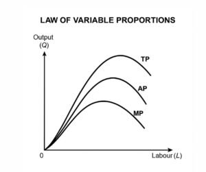
UGC NET Economics Unit 1-General Equilibrium Analysis

1. Introduction

The concept of general equilibrium represents one of the core analytical tools in microeconomics. While partial equilibrium examines individual markets in isolation, general equilibrium analysis studies the simultaneous equilibrium of all interrelated markets — goods, services, and factors — within an economy.

This framework was developed by Léon Walras, whose Elements of Pure Economics (1874) provided the mathematical foundation for modern equilibrium theory. His approach, known as the Walrasian General Equilibrium Model, remains the cornerstone of equilibrium analysis.

2. Partial vs. General Equilibrium

Partial Equilibrium Analysis

Introduced by Alfred Marshall, this method isolates one market or variable while assuming all others remain constant (ceteris paribus).
It is suitable for studying specific issues like:
- Demand and supply in a single commodity market.
- Price determination in isolation.
Limitations:
- Ignores interdependence between markets.
- Assumes other prices, incomes, and tastes remain unchanged.

General Equilibrium Analysis

Developed by Walras, this approach considers simultaneous interaction of all markets.
It acknowledges that a change in one market affects others (e.g., a rise in food prices affects wages, cost of production, and factor markets).
Objective: To determine whether a set of prices exists that brings equilibrium in all markets simultaneously.

3. Walrasian General Equilibrium Model

Assumptions

Perfect competition in all markets.
Rational consumers maximize utility; firms maximize profits.
Factors and goods are homogeneous and perfectly divisible.
All markets clear — supply equals demand.

Structure of the Model

Suppose the economy has:

n commodities, m factors, and h households.

Each market has:

Demand functions: $Q_{i}^{d} = D_{i} (P_{1}, P_{2}, . . ., P_{n}, M_{1}, M_{2}, . . ., M_{h})$
Supply functions: $Q_{i}^{s} = S_{i} (P_{1}, P_{2}, . . ., P_{n}, V_{1}, V_{2}, . . ., V_{m})$
Factor demand functions: $R_{k}^{d} = D_{k} (Q_{1}, . . ., Q_{n}, P_{1}, . . ., P_{n}, V_{1}, . . ., V_{m})$
Factor supply functions: $R_{k}^{s} = S_{k} (V_{1}, V_{2}, . . ., V_{m}; R_{k 1}, R_{k 2}, . . ., R_{k h})$

Walras’ Law

The sum of excess demands across all markets is zero:

\sum (P_i Q_i^d – P_i Q_i^s) = 0
]
This means that if all but one market are in equilibrium, the last one must also be in equilibrium.

4. Graphical Illustration (2×2×2 Model)

Consider:

2 goods (X and Y)
2 factors (Labour L and Capital K)
2 consumers (A and B)

When demand for one good (say X) rises:

Price of X rises → firms in X earn supernormal profits.
Resources (L, K) move from industry Y to X.
Price of Y falls → firms in Y incur losses.
Over time, this reallocation of resources restores equilibrium across both goods and factor markets.

This automatic adjustment mechanism demonstrates how the market tends toward general equilibrium.

5. Existence, Uniqueness, and Stability of General Equilibrium

1️⃣ Existence

A general equilibrium exists if a set of prices makes aggregate demand = aggregate supply in all markets.

Walras proved existence mathematically using simultaneous equations.
Modern proofs (Arrow–Debreu, 1954) showed equilibrium exists under:
- Convex preferences,
- Continuous, decreasing returns to scale,
- No externalities.

2️⃣ Uniqueness

Equilibrium is unique if there is only one set of prices that clears all markets.

Uniqueness requires:
- Strict convexity of preferences,
- Non-intersecting excess demand curves.
If demand curves are backward-bending (as in Giffen goods), multiple equilibria can exist.

3️⃣ Stability

An equilibrium is stable if deviations from it trigger market forces that restore equilibrium.

Stable Equilibrium: When market adjustment brings the system back (demand < supply → prices fall → equilibrium restored).
Unstable Equilibrium: Divergence from equilibrium continues.
Stability depends on relative slopes of demand and supply curves and adjustment mechanisms.

6. Pareto Efficiency and General Equilibrium

A general equilibrium is Pareto efficient when no reallocation of resources can make someone better off without making someone else worse off.

Conditions for Pareto Optimality:

Efficiency in Consumption:
- MRS (A) = MRS (B)
Efficiency in Production:
- MRTS (X) = MRTS (Y)
Efficiency in Product Mix:
- MRT (production) = MRS (consumption)

When these three conditions are met, the economy achieves Pareto optimality.

7. Extensions of General Equilibrium

Kaldor–Hicks Efficiency: Improvement is efficient if gainers could compensate losers.
Social Welfare Function (Bergson–Samuelson): Aggregates individual preferences into a measure of societal welfare.
Second Welfare Theorem: Any Pareto optimal allocation can be achieved through appropriate redistribution and competitive equilibrium.

8. Limitations of General Equilibrium Analysis

Assumes perfect competition, rarely observed in reality.
Neglects time-lags and dynamic processes.
Requires complete information and rationality.
Ignores externalities and public goods.
Complex mathematical modeling limits empirical application.

9. Key Terms

Concept	Description
Partial Equilibrium	Analysis of one market in isolation.
General Equilibrium	Simultaneous equilibrium in all markets.
Walrasian System	A system of simultaneous equations determining all prices and quantities.
Pareto Optimality	Resource allocation where no one can be made better off without hurting another.
Walras’ Law	If all but one markets are in equilibrium, the last one must also be.
Stability	The tendency of a system to return to equilibrium after a disturbance.

10. Summary for UGC NET Preparation

Distinguish between Partial and General Equilibrium.
Understand Walrasian Model and Walras’ Law.
Learn the conditions of existence, uniqueness, and stability.
Relate General Equilibrium to Welfare Economics (Pareto, Kaldor–Hicks).
Review the Arrow–Debreu model for modern proofs.
Remember diagrams for 2×2×2 model, Edgeworth Box, and Production Possibility Frontier.

General Equilibrium Analysis (Extended Notes with Edgeworth Box & Pareto Efficiency)

(UGC NET Economics – Unit 1: Microeconomics)

1. Introduction to the Edgeworth Box

The Edgeworth Box Diagram is one of the most important tools for understanding General Equilibrium and Pareto Efficiency in both exchange and production.

It was developed by Francis Ysidro Edgeworth (1881) and later refined by Vilfredo Pareto (1906).

The Edgeworth Box provides a graphical representation of a two-person, two-good economy, showing how resources or goods can be distributed between two individuals (or firms) to achieve efficient allocations.

2. Structure of the Edgeworth Box

Assumptions:

Two consumers (A and B)
Two goods (X and Y)
Fixed total quantities of X and Y
$X_{A} + X_{B} = \overset{ˉ}{X}, Y_{A} + Y_{B} = \overset{ˉ}{Y}$
Preferences of both consumers are convex, continuous, and represented by indifference curves.
There is no production — only exchange.

Diagram Description

Imagine a rectangle (the box):

The width of the box represents the total quantity of good X available.
The height represents the total quantity of good Y.
The origin for consumer A is at the bottom-left corner (Oₐ).
The origin for consumer B is at the top-right corner (Oᵦ).

Each point inside the box represents one possible distribution of goods X and Y between A and B.

Indifference Curves

ICₐ = Indifference curves of consumer A (convex to Oₐ).
ICᵦ = Indifference curves of consumer B (convex to Oᵦ).
The point of tangency between ICₐ and ICᵦ shows a state where both consumers cannot be made better off without hurting the other — a Pareto efficient allocation.

3. The Contract Curve

Definition:

The Contract Curve is the locus of all tangency points between the indifference curves of A and B inside the Edgeworth Box.

It represents all Pareto Efficient (optimal) allocations of the two goods between the two individuals.

Mathematical Condition:

At Pareto Efficiency, the Marginal Rate of Substitution (MRS) of both individuals must be equal:

$M R S_{X Y}^{A} = M R S_{X Y}^{B}$

That is,

$\frac{M U_{X}^{A}}{M U_{Y}^{A}} = \frac{M U_{X}^{B}}{M U_{Y}^{B}}$

When this condition holds, neither A nor B can be made better off without making the other worse off.

Interpretation:

Every point on the Contract Curve is Pareto Efficient, but not all points are socially desirable.
The final outcome depends on initial endowments and bargaining power (see the core of exchange below).

4. The Core of Exchange

The Core is the subset of Pareto-efficient points on the contract curve that both individuals prefer over their initial endowment.
It represents the possible range of mutually beneficial trades.

Thus:

$Core \subset Contract Curve$

At any point outside the core, one or both individuals would reject the trade.

5. Edgeworth Box for Production

In the production version of the Edgeworth Box:

Consumers are replaced by firms.
Goods X and Y are replaced by two factors of production (Labour L and Capital K).
Isoquants represent combinations of inputs (L, K) producing the same output.

Production Efficiency Condition:

For efficiency in production,

$M R T S_{L K}^{X} = M R T S_{L K}^{Y}$

That is, the Marginal Rate of Technical Substitution between labour and capital must be equal for both industries.

This ensures that no reallocation of resources can increase total output of one good without reducing that of another.

6. Combining Exchange and Production: The General Equilibrium

Once efficiency in production and efficiency in exchange are achieved, we combine both through the Production Possibility Frontier (PPF) and the Community Indifference Curve (CIC).

Efficiency in Product Mix:

$M R T_{X Y} = M R S_{X Y}$

Where:

MRT = Marginal Rate of Transformation (slope of PPF)
MRS = Marginal Rate of Substitution (slope of CIC)

This ensures the optimal combination of goods produced matches the pattern of consumers’ preferences.

🧮 7. Three Conditions for Pareto Efficiency

Type of Efficiency	Condition	Meaning
Efficiency in Exchange	$M R S_{X Y}^{A} = M R S_{X Y}^{B}$	Goods are allocated efficiently among consumers.
Efficiency in Production	$M R T S_{L K}^{X} = M R T S_{L K}^{Y}$	Factors are optimally allocated among producers.
Efficiency in Product Mix	$M R S_{X Y} = M R T_{X Y}$	Output mix matches consumers’ preferences.

When all three hold simultaneously, the economy is in general equilibrium and Pareto efficient.

8. Graphical Summary

The Edgeworth Box (Exchange) shows efficient distribution of goods between consumers.
The Edgeworth Box (Production) shows efficient allocation of factors among firms.
The PPF–CIC Framework shows efficient combination of goods matching social preferences.

These three layers together form the General Equilibrium Model of the economy.

9. Welfare Theorems and General Equilibrium

First Fundamental Theorem of Welfare Economics

Under perfect competition, every general equilibrium allocation is Pareto Efficient.

Second Fundamental Theorem of Welfare Economics

Any Pareto Efficient allocation can be achieved by suitable redistribution of initial endowments and then allowing competitive equilibrium.

This implies that equity and efficiency can be separated — government can redistribute endowments without distorting market efficiency.

10. Key Takeaways for UGC NET

Concept	Key Formula / Condition	UGC NET Focus
General Equilibrium	All markets clear simultaneously	Difference from partial equilibrium
Walras’ Law	∑(Excess Demand × Price) = 0	Importance for equilibrium
Pareto Efficiency	No reallocation can improve welfare of one without hurting another	Concept of welfare optimality
Contract Curve	MRSₐ = MRSᵦ	Set of all efficient allocations
Production Efficiency	MRTS_x = MRTS_y	Optimal use of factors
Product-Mix Efficiency	MRS = MRT	Equilibrium between production and consumption
First & Second Welfare Theorems	Competitive equilibrium ↔ Pareto efficiency	Role of redistribution

November 2, 2025

UGC NET Economics Unit-1-Factor Pricing-MCQs

UGC NET ECONOMICS: FACTOR PRICING

1.

Factor pricing theory is also known as:
A) Theory of Value
B) Theory of Cost
C) Theory of Distribution
D) Theory of Exchange
Answer: C

2.

The Marginal Productivity Theory states that each factor is paid:
A) The total value of its contribution
B) According to its marginal product
C) According to average productivity
D) A fixed wage rate
Answer: B

3.

According to Marginal Productivity Theory, a firm is in equilibrium when:
A) $M R P = M F C$
B) $M R = M C$
C) $A R = A C$
D) $M F C = M P$
Answer: A

4.

Under perfect competition, the equilibrium condition in factor markets is:
A) $M R P = M F C = P_{f}$
B) $M R P > M F C$
C) $M F C = 0$
D) $P_{f} > M R$
Answer: A

5.

Value of Marginal Product (VMP) equals:
A) $M P \times M R$
B) $M P \times P r i c e$
C) $M R - M C$
D) $M P / P r i c e$
Answer: B

6.

When product market is imperfect, the relationship between VMP and MRP is:
A) $V M P = M R P$
B) $V M P < M R P$
C) $V M P > M R P$
D) $V M P = 0$
Answer: C

7.

The demand for a factor is:
A) Autonomous
B) Independent
C) Derived demand
D) Complementary demand
Answer: C

8.

Which of the following is not an assumption of the Marginal Productivity Theory?
A) Perfect competition
B) Homogeneous factors
C) Imperfect knowledge
D) Full employment
Answer: C

9.

The Marginal Revenue Product (MRP) of a factor is the:
A) Additional output per extra unit of factor
B) Extra revenue earned from one more unit of factor
C) Average revenue per unit of factor
D) Price per unit of factor
Answer: B

10.

The Marginal Productivity Theory was refined and popularized by:
A) Ricardo and Mill
B) Marshall and Clark
C) Adam Smith and Keynes
D) Hicks and Kaldor
Answer: B

11.

The Modern Theory of Factor Pricing determines factor prices by:
A) Productivity alone
B) Supply of factors alone
C) Interaction of demand and supply of factors
D) Government intervention
Answer: C

12.

When $M R P < M F C$ , a profit-maximizing firm should:
A) Employ more of the factor
B) Reduce employment of the factor
C) Keep employment constant
D) Increase factor price
Answer: B

13.

Under monopsony in a labour market, equilibrium occurs when:
A) $W = M R P L$
B) $M F C = M R P L$
C) $W > M R P L$
D) $W = M F C$
Answer: B

14.

Under monopsony, the wage rate is:
A) Higher than in perfect competition
B) Equal to MRP
C) Lower than in perfect competition
D) Always zero
Answer: C

15.

The Ricardian Theory of Rent assumes that rent arises due to:
A) Scarcity of land
B) Fertility differences among lands
C) Monopoly power
D) Labour productivity
Answer: B

16.

According to Ricardo, no-rent land refers to:
A) The most fertile land
B) The least fertile land under cultivation
C) Unused barren land
D) Land with highest productivity
Answer: B

17.

Economic rent is:
A) Payment to land only
B) Surplus over opportunity cost
C) Equal to transfer earnings
D) Dependent on sunk costs
Answer: B

18.

The Modern Theory of Rent (Scarcity Rent) was proposed by:
A) David Ricardo
B) Marshall
C) Hicks
D) Robbins
Answer: B

19.

The Subsistence Theory of Wages was given by:
A) J.S. Mill
B) Ricardo
C) David Ricardo and Lassalle
D) Adam Smith
Answer: C

20.

According to Marginal Productivity Theory of Wages, the wage rate equals:
A) Average productivity of labour
B) Marginal revenue productivity of labour
C) Total revenue divided by number of workers
D) Wage fund per worker
Answer: B

21.

The Loanable Funds Theory explains the determination of:
A) Rent
B) Wage
C) Interest rate
D) Profit
Answer: C

22.

According to Loanable Funds Theory, the rate of interest is determined by:
A) Demand and supply of loanable funds
B) Marginal productivity of capital
C) Government policy
D) Saving alone
Answer: A

23.

The Keynesian Liquidity Preference Theory suggests that:
A) Interest is reward for saving
B) Interest is reward for productivity
C) Interest is reward for parting with liquidity
D) Interest equals rate of return on capital
Answer: C

24.

According to Knight’s Risk Theory, profit is:
A) A reward for innovation
B) A return for bearing uncertainty
C) A payment for management
D) A premium on capital
Answer: B

25.

According to Schumpeter’s Innovation Theory, profit arises due to:
A) Monopoly power
B) Risk-taking
C) Innovations and technological changes
D) Labour productivity
Answer: C

26.

In general equilibrium, factor prices are determined:
A) Independently in each market
B) Simultaneously in all markets
C) By the government only
D) By consumer preferences
Answer: B

27.

In a perfectly competitive factor market, the supply curve of a factor is:
A) Perfectly elastic
B) Perfectly inelastic
C) Backward bending
D) Upward sloping
Answer: A

28.

Under imperfect product markets, the MRP curve lies:
A) Above VMP curve
B) Below VMP curve
C) Coincides with VMP curve
D) Equal to average cost curve
Answer: B

29.

When demand for labour increases while supply remains constant, equilibrium wage will:
A) Fall
B) Rise
C) Remain same
D) Become negative
Answer: B

30.

In a bilateral monopoly (one buyer and one seller of labour), wages are determined by:
A) Government policy
B) Collective bargaining
C) Marginal productivity
D) Random negotiation
Answer: B

November 1, 2025

UGC NET Economics Unit 1-Factor Pricing

(Unit 1 – Microeconomics)
Based on the UGC NET Economics syllabus and referenced from your uploaded MA Microeconomics textbook.

1. Introduction to Factor Pricing

Factor pricing deals with how the rewards (prices) of factors of production—land, labour, capital, and entrepreneurship—are determined in the factor market.
These rewards are:

Factor	Reward
Land	Rent
Labour	Wages
Capital	Interest
Entrepreneurship	Profit

Thus, factor pricing theory is also known as the theory of distribution because it explains how the national income is distributed among the different factors of production.

2. Meaning and Scope

The study of factor pricing focuses on:

Determining the price (remuneration) of each factor.
Understanding factor demand and supply.
Explaining functional distribution (income distribution among factors).
Analysing market imperfections and their effect on factor earnings.

It answers:

Why do workers receive different wages?
Why is rent earned by land?
Why does capital earn interest?
Why do entrepreneurs make profits or incur losses?

3. Theories of Factor Pricing

There are two broad approaches:

A. Macro Theory of Distribution

Deals with total national income and its division among the factors.
Concerned with the shares of wages, rent, interest, and profit in national income.
Example: Ricardian distribution theory.

B. Micro Theory of Distribution

Deals with the reward of a particular factor in a specific industry.
Example: Marginal Productivity Theory of Distribution.

4. Marginal Productivity Theory of Distribution

This is the most prominent theory of factor pricing.

Assumptions

Perfect competition in product and factor markets.
Homogeneous factors.
Perfect mobility of factors.
Full employment.
Diminishing marginal productivity.
Profit-maximizing firm.

Concept

A rational firm will employ a factor up to the point where:

$Marginal Revenue Product (MRP) = Marginal Factor Cost (MFC)$

In a perfectly competitive factor market:

$M F C = P r i c e (of the factor)$

Thus, equilibrium occurs when:

$MRP = Factor Price$

Diagrammatic Explanation

![MRP Curve](conceptual representation)

The MRP curve is downward-sloping due to diminishing marginal productivity.
The MFC line (wage rate or factor price) is horizontal under perfect competition.
The intersection determines equilibrium employment and factor price.

Mathematical Expression

$M R P = M P \times M R$

Under perfect competition, $M R = P$ , so:

$M R P = M P \times P$

Hence, factor price = MRP at equilibrium.

Implications

Every factor is paid according to its contribution to production.
Explains both demand and price determination for factors.
Income distribution is based on productivity, not exploitation.

5. Concepts Related to Marginal Productivity Theory

Concept	Meaning
Average Product (AP)	Output per unit of factor employed.
Marginal Product (MP)	Additional output from one more unit of factor.
Value of Marginal Product (VMP)	MP × Price of output.
Marginal Revenue Product (MRP)	MP × Marginal Revenue (under imperfect competition).
Marginal Factor Cost (MFC)	Additional cost from employing one more unit of a factor.

Under perfect competition:

$V M P = M R P = F a c t o r P r i c e$

6. Criticisms of Marginal Productivity Theory

Unrealistic assumptions (perfect competition rarely exists).
Circular reasoning – price of factor depends on product price, which depends on cost, which again depends on factor prices.
Static model – ignores time and technological changes.
Immobility of factors in reality.
Non-measurable productivity for collective factors (e.g., teamwork).

Despite these, the theory is foundational and forms the basis of modern factor pricing models.

7. Modern Theory of Factor Pricing

The modern approach integrates both demand and supply of factors.
A factor’s price is determined by the interaction of its demand (MRP) and supply.

Equilibrium Condition:

$D_{f} = S_{f}$

where
$D_{f}$ = Demand for factor (MRP curve)
$S_{f}$ = Supply of factor (upward sloping)

The intersection gives the equilibrium factor price (wage, rent, interest, or profit).

Determination of Factor Price

Market Condition	Outcome
Perfect competition (factor & product)	$M R P = M F C = P$
Imperfect product market	$P > M R$ , so $M R P < V M P$
Imperfect factor market	$M F C > w a g e$ , so lower employment

8. Theories of Individual Factor Pricing

A. Rent (Land) – Ricardian Theory of Rent

Rent arises due to differences in fertility of land.
Rent = Surplus over the cost of cultivation on the marginal land.

$Economic Rent = Total Revenue - Total Cost$

B. Wages (Labour) – Marginal Productivity Theory & Modern Theories

Wages determined where:

$M R P_{L} = W$

Under monopoly, wages may be below MRP.
Modern extensions include bargaining, efficiency wage, and labour union effects.

C. Interest (Capital) – Classical and Modern Theories

Classical Theory: Interest determined by demand (investment) and supply (saving).
Loanable Funds Theory: Interest = interaction of demand and supply of loanable funds.
Keynesian Theory: Interest determined by liquidity preference and money supply.

$i = f (L P, M)$

D. Profit (Entrepreneurship) – Risk and Innovation Theories

Risk Theory (Knight): Profit is a reward for bearing uncertainty.
Innovation Theory (Schumpeter): Profit arises due to innovation and entrepreneurial dynamism.
Dynamic Theory: Profit results from changes in demand, technology, and organisation.

9. Modern View: General Equilibrium of Factor Markets

Using Walrasian General Equilibrium, all factor prices are interdependent:

Each factor’s demand depends on product demand.
Product price depends on factor costs.
Hence, equilibrium requires simultaneous determination of all factor prices.

Mathematically, equilibrium is achieved when:

$\sum_{i} D_{i} = \sum_{i} S_{i} for all factors i$

10. Efficiency and Welfare Implications

Efficiency Type	Factor Market Condition	Achieved When
Allocative Efficiency	$P_{f a c t o r} = M R P$	Yes (Perfect Competition)
Distributive Efficiency	Each factor paid according to productivity	Yes
Pareto Optimality	No reallocation can improve welfare	Achieved in equilibrium

11. Factor Pricing under Imperfect Competition

Type	Key Features	Outcome
Monopsony in Labour Market	Single buyer of labour	$M F C > W a g e$ ; lower employment
Monopoly in Product Market	$M R < P$ ; $M R P < V M P$	Lower factor demand
Bilateral Monopoly	Single buyer & single seller	Wage set through bargaining
Oligopsony	Few buyers	Wages depressed below competitive level

12. Summary Table

Factor	Classical Theory	Modern/Keynesian Theory	Key Determinant
Land (Rent)	Differential fertility (Ricardo)	Scarcity rent	Productivity & scarcity
Labour (Wages)	Subsistence & marginal productivity	Demand-supply equilibrium	Productivity & bargaining
Capital (Interest)	Abstinence (saving)	Liquidity preference	Supply of money & savings
Entrepreneur (Profit)	Risk & uncertainty	Innovation & monopoly power	Change, risk, innovation

13. UGC NET Focus Areas

Subtopic	Weightage	Concepts to Master
Marginal Productivity Theory	25%	$M R P = M F C$ , efficiency
Rent Theories	20%	Ricardian & scarcity rent
Wage Determination	20%	Competitive vs monopsony
Interest & Profit	20%	Loanable funds, innovation theory
General Equilibrium of Factor Markets	15%	Pareto efficiency

14. Key Takeaways

Factor pricing explains income distribution across productive agents.
Marginal productivity is the cornerstone of classical and neoclassical thought.
Modern theories integrate demand and supply to form realistic explanations.
Market imperfections (monopoly, monopsony, unions) alter equilibrium prices.
Efficient factor markets ensure Pareto optimal allocation of resources.

November 1, 2025

UGC NET Economics UNIT 1-MARKET STRUCTURES AND EFFICIENCY-MCQs

1.

In perfect competition, each firm is a:
A) Price maker
B) Price taker
C) Quantity setter
D) Collusive participant
Answer: B

2.

Under perfect competition, a firm attains equilibrium where:
A) $A R = A C$
B) $M C = M R$
C) $M C > M R$
D) $T R = T C$

Answer: B

3.

In long-run equilibrium under perfect competition, which holds true?
A) $P = M C = A C = M R$
B) $P > M C$
C) $P < A C$
D) $P > M R$
Answer: A

4.

Allocative efficiency is achieved when:
A) $P > M C$
B) $P < M C$
C) $P = M C$
D) $M R = M C$
Answer: C

5.

Which of the following ensures productive efficiency?
A) Output is maximized.
B) Production occurs at minimum AC.
C) Firms make zero profit.
D) $M C = M R$
Answer: B

6.

A monopolist faces a downward-sloping demand curve because:
A) Entry barriers are low.
B) It produces homogeneous products.
C) It is the sole producer with no substitutes.
D) It acts as a price taker.
Answer: C

7.

In monopoly equilibrium:
A) $P = M C$
B) $P = M R$
C) $P > M R = M C$
D) $P = A C = M C$
Answer: C

8.

Which one is true for perfect competition but not for monopoly?
A) $P = M C$
B) Downward-sloping demand curve
C) Entry barriers exist
D) Firm determines price
Answer: A

9.

The condition $P > M C$ under monopoly implies:
A) Allocative efficiency
B) Productive efficiency
C) Welfare loss
D) Increasing returns to scale
Answer: C

10.

The deadweight loss in monopoly arises due to:
A) Perfect knowledge
B) Overproduction
C) Restriction of output
D) Constant returns to scale
Answer: C

11.

The Lerner Index measures:
A) Profit rate
B) Monopoly power
C) Efficiency loss
D) Output elasticity
Answer: B

$L = \frac{P - M C}{P}$

12.

Which of the following market structures shows zero long-run economic profit?
A) Monopoly
B) Oligopoly
C) Monopolistic Competition
D) Duopoly
Answer: C

13.

In monopolistic competition, each firm faces:
A) Perfectly elastic demand curve
B) Downward-sloping demand curve
C) Perfectly inelastic demand curve
D) Horizontal marginal revenue curve
Answer: B

14.

The key feature distinguishing monopolistic competition from perfect competition is:
A) Entry restrictions
B) Product differentiation
C) Price control
D) Number of firms
Answer: B

15.

Under monopolistic competition, the firm achieves equilibrium when:
A) $M C = M R$ and $P = M C$
B) $M C = M R$ and $P > M C$
C) $M C = M R = A C$
D) $M R = A R$
Answer: B

16.

Which of the following statements is true for long-run equilibrium in monopolistic competition?
A) Firms earn supernormal profits.
B) Firms produce at minimum AC.
C) Firms earn normal profits but not at minimum AC.
D) Price equals MC.
Answer: C

17.

Excess capacity in monopolistic competition arises because:
A) Firms overproduce
B) Entry is restricted
C) Firms produce less than optimal scale of output
D) Price equals MC
Answer: C

18.

In oligopoly, firms are:
A) Independent in pricing
B) Interdependent in pricing
C) Non-profit-maximizing
D) Price takers
Answer: B

19.

Which of the following is a model of oligopoly?
A) Cournot Model
B) Walrasian Model
C) Arrow-Debreu Model
D) Ricardian Model
Answer: A

20.

In Cournot Duopoly, each firm assumes that the rival’s output:
A) Will remain constant
B) Will increase proportionally
C) Will decrease as own output increases
D) Is unknown
Answer: A

21.

In Bertrand Competition, firms compete by choosing:
A) Output levels
B) Prices
C) Market shares
D) Advertising levels
Answer: B

22.

The Kinked Demand Curve model of oligopoly explains:
A) Price discrimination
B) Sticky prices
C) Collusion
D) Entry barriers
Answer: B

23.

Price rigidity in the kinked demand model arises because:
A) Marginal cost fluctuates
B) Firms fear rival reactions to price changes
C) Demand is perfectly elastic
D) Firms have identical costs
Answer: B

24.

A collusive oligopoly tends to behave like:
A) Perfect competition
B) Monopoly
C) Duopoly
D) Monopolistic competition
Answer: B

25.

Allocative inefficiency is present when:
A) $P = M C$
B) $P > M C$
C) $M C > M R$
D) $A R = M R$
Answer: B

26.

In long-run equilibrium under perfect competition, welfare is:
A) Maximized
B) Reduced
C) Constant
D) Uncertain
Answer: A

27.

Dynamic efficiency is most likely to occur in:
A) Perfect competition
B) Monopoly and oligopoly
C) Monopolistic competition
D) Duopoly only
Answer: B

🟩 Because large profits can fund R&D and innovation.

28.

The deadweight loss triangle in monopoly represents:
A) Excess profit
B) Lost consumer and producer surplus
C) Minimum efficiency output
D) Social gain
Answer: B

29.

Which market structure shows both competition and differentiation?
A) Monopoly
B) Oligopoly
C) Monopolistic Competition
D) Perfect Competition
Answer: C

30.

When the government regulates a natural monopoly, its aim is usually to:
A) Maximize monopolist’s profit
B) Reduce consumer surplus
C) Bring $P$ closer to $M C$
D) Restrict entry further
Answer: C

November 1, 2025

UGC NET Economics Unit 1-Market Structures, Competitive and Non-Competitive Equilibria, and Their Efficiency Properties

(Unit 1 – Microeconomics)

1. Introduction

The concept of market structure refers to the nature and degree of competition prevailing in a particular market or industry. It is defined by characteristics such as number of firms, nature of the product, entry and exit conditions, market power, and price control.

Market structures influence how firms behave, determine equilibrium prices and outputs, and affect economic efficiency and welfare.

2. Classification of Market Structures

Market Structure	No. of Sellers	Type of Product	Price Control	Entry/Exit Barriers
Perfect Competition	Many	Homogeneous	None	Free
Monopolistic Competition	Many	Differentiated	Limited	Free
Oligopoly	Few	Homogeneous/Differentiated	Considerable	High
Monopoly	One	Unique	Absolute	Very High

Each market structure leads to a different price-output determination and distinct efficiency outcomes.

3. Perfect Competition

Characteristics

Large number of buyers and sellers
Homogeneous product
Perfect knowledge
Free entry and exit
Perfect mobility of factors
Firms are price takers

Short-Run Equilibrium

A firm is in equilibrium when:

$M C = M R$

and the MC curve cuts the MR curve from below.

Depending on cost and price levels, the firm may earn supernormal profits, normal profits, or losses.

Long-Run Equilibrium

In the long run, entry and exit of firms drive all firms to earn normal profits.

$P = M C = M R = A R = A C$

This represents productive and allocative efficiency.

Efficiency under Perfect Competition

Type of Efficiency	Explanation	Achieved?
Allocative Efficiency	$P = M C$ ensures resources are optimally allocated.	✅ Yes
Productive Efficiency	Firms produce at minimum AC.	✅ Yes
Dynamic Efficiency	Innovation over time.	⚙️ Moderate
Distributive Efficiency	No exploitation of consumers.	✅ Yes

Thus, perfect competition is socially optimal.

4. Monopoly

Features

Single seller and no close substitutes
Barriers to entry
Price maker
Firm = Industry

Equilibrium

$M C = M R$

but price (P) > MC, since the monopolist faces a downward-sloping demand curve.

Condition	Implication
$M R = M C$	Profit maximization
$P > M R$	Market power
$P > M C$	Allocative inefficiency

Welfare Implications

Monopoly leads to:

Higher price and lower output than perfect competition.
Deadweight loss (DWL) due to misallocation of resources.

Efficiency under Monopoly

Efficiency Type	Status	Reason
Allocative Efficiency	❌	$P > M C$ → underproduction
Productive Efficiency	❌	X-inefficiency due to lack of competition
Dynamic Efficiency	⚙️ Sometimes achieved	Large profits may fund R&D
Distributive Efficiency	❌	Consumer surplus transferred to producer

5. Monopolistic Competition

Features

Many sellers, product differentiation
Freedom of entry and exit
Some control over price
Heavy non-price competition (advertising, branding)

Equilibrium

Each firm faces a downward-sloping demand curve (AR).
In equilibrium:

$M C = M R$

but

$P > M C$

In the long run, new entrants eliminate supernormal profits → only normal profits remain.

Efficiency

Allocative Inefficiency: $P > M C$
Productive Inefficiency: Firms don’t produce at minimum AC
Excess Capacity: Output is below optimum scale

However, variety and consumer choice increase welfare partially.

6. Oligopoly

Features

Few large firms dominate
Mutual interdependence
Product differentiation (or homogeneity)
Entry barriers
Strategic behaviour (Game theory relevance)

Models of Oligopoly

Model	Description	Key Outcome
Cournot Duopoly	Firms choose quantities simultaneously	Intermediate output
Bertrand Model	Firms compete in prices	Price = MC (competitive outcome)
Sweezy’s Kinked Demand Curve	Price rigidity; firms reluctant to change prices	Sticky prices
Collusive Oligopoly	Firms cooperate via cartel	Monopoly-like price

Efficiency

Allocative Efficiency: Not achieved; $P > M C$
Productive Efficiency: Not achieved; high AC due to inefficiency
Dynamic Efficiency: Often high (innovation driven by rivalry)

7. Comparative Equilibrium Analysis

Feature	Perfect Competition	Monopoly	Monopolistic Competition	Oligopoly
Price	Lowest	Highest	Moderate	Moderate–High
Output	Highest	Lowest	Less than PC	Less than PC
Entry	Free	Blocked	Free	Restricted
Profit (Long Run)	Normal	Abnormal	Normal	May persist
Efficiency	High	Low	Moderate	Mixed

8. Efficiency Properties and Welfare Implications

A. Allocative Efficiency

Achieved when $P = M C$ → society values goods as much as they cost to produce.
Only perfect competition satisfies this condition.

B. Productive Efficiency

Achieved when firms produce at minimum AC.
Only perfect competition attains this in the long run.

C. Dynamic Efficiency

Relates to technological innovation and R&D investment.
Often higher in monopolistic and oligopolistic markets due to profit incentives.

D. X-Inefficiency

Monopoly and oligopoly may exhibit inefficiency due to slack management.

E. Welfare and Deadweight Loss

Deadweight loss under monopoly or oligopoly arises because:

$P > M C \Rightarrow Q_{m} < Q_{c}$

— representing lost consumer and producer surplus.

9. Competitive vs. Non-Competitive Equilibria

Criterion	Competitive Markets	Non-Competitive Markets
Price Determination	Market demand & supply	Firm’s market power
Output	Efficient allocation	Restricted output
Profit	Normal	Supernormal
Entry/Exit	Free	Restricted
Welfare	Maximized	Reduced
Market Power	None	Present

10. Efficiency and Market Failure

Market Failure Causes

Monopoly power (restrictive output, higher prices)
Externalities
Public goods
Asymmetric information

When markets fail to achieve Pareto optimality, government intervention (regulation, taxation, antitrust) may restore efficiency.

11. Policy Implications

Promote Competition: Encourage entry and discourage collusion.
Antitrust Laws: Prevent monopoly abuse.
Regulation: Control prices in natural monopolies (utilities).
Subsidies for R&D: Enhance dynamic efficiency.
Public Provision: Where private markets fail (education, healthcare).

12. Summary

Concept	Key Points
Market Structure	Framework defining number and behaviour of firms
Perfect Competition	Maximizes welfare, allocative and productive efficiency
Monopoly	Leads to deadweight loss and inefficiency
Monopolistic Competition	Product variety with some inefficiency
Oligopoly	Interdependence and strategic behaviour dominate
Efficiency Properties	Only perfect competition ensures Pareto efficiency
Policy Measures	Needed to correct market failures in non-competitive equilibria

13. Visual Summary (for Diagrams)

Perfect Competition: $P = M C = M R$ , lowest price, highest output.
Monopoly: $P > M C$ , restricted output, deadweight loss.
Monopolistic Competition: $P > M C$ , excess capacity.
Oligopoly: Price rigidity, interdependent demand curves.

14. UGC NET Focus Areas

Subtopic	Expected Weightage	Common Questions
Perfect vs Imperfect Markets	25%	Price & output equilibrium
Efficiency Conditions	25%	$P = M C$ , $A C = M C$
Monopoly Welfare Loss	20%	Deadweight triangle analysis
Oligopoly Models	15%	Cournot, Bertrand, Kinked demand
Market Failure & Regulation	15%	Policy implications

15. Key Takeaway

Perfect competition is the benchmark for maximum efficiency.
All non-competitive structures—monopoly, monopolistic competition, and oligopoly—deviate from Pareto optimality, leading to welfare loss.
However, dynamic gains in innovation may sometimes justify moderate market power.

November 1, 2025

UGC NET Economics Unit 1 – Game Theory – Non-Cooperative Games

(Based on “MA Microeconomics” textbook and UGC NET syllabus)

1. Introduction

Game Theory is a mathematical framework that analyzes strategic interactions among rational decision-makers (players), where the outcome of one’s decision depends on the choices of others.

It was first formalized by John von Neumann and Oskar Morgenstern in their classic book Theory of Games and Economic Behavior (1944).

In Microeconomics, Game Theory is particularly useful in studying oligopolistic markets, where few firms make interdependent decisions regarding price, output, and advertising.

2. Classification of Games

Basis	Types	Explanation
Number of Players	Two-player, n-player	Duopoly, Oligopoly, etc.
Nature of Payoffs	Zero-sum, Non-zero-sum	In zero-sum, one’s gain = another’s loss.
Nature of Cooperation	Cooperative, Non-cooperative	Cooperative involves binding agreements; non-cooperative involves independent strategies.
Timing of Moves	Simultaneous, Sequential	Firms act together or one after another.
Information Availability	Complete, Incomplete	Players may or may not know each other’s payoffs.

3. Non-Cooperative Games: Meaning and Features

A non-cooperative game is one where players make decisions independently, without collaboration or binding agreements.
Each player selects a strategy that maximizes their own payoff, given their beliefs about others’ choices.

Features

Independent decision-making
Strategic interdependence
Use of payoff matrices
Focus on Nash Equilibrium
May involve dominant or mixed strategies

4. Basic Concepts of Non-Cooperative Games

A. Players and Strategies

Players: The decision-makers (e.g., firms in oligopoly).
Strategies: Plans of action available to each player (e.g., “Raise Price” or “Cut Price”).
Payoff: The reward or outcome for each combination of strategies.

A payoff matrix shows all possible outcomes.

B. Payoff Matrix (Example)

Firm B ↓ / Firm A →	High Price	Low Price
High Price	(10, 10)	(2, 15)
Low Price	(15, 2)	(5, 5)

Each cell shows the profits (A, B) from their chosen strategies.

5. Dominant Strategy

A dominant strategy is one that provides a higher payoff to a player, regardless of what others do.

Example:

If Firm A earns higher profit by always choosing “Low Price,” then “Low Price” is its dominant strategy.

If both firms have dominant strategies, the resulting outcome is called the Dominant Strategy Equilibrium.

6. Nash Equilibrium

Introduced by John Nash (1950), the Nash Equilibrium occurs when no player can improve their payoff by unilaterally changing their strategy, given the other’s choice.

In the above payoff matrix:

(Low Price, Low Price) = (5, 5)
Neither A nor B gains by changing strategy → Nash Equilibrium.

7. The Prisoner’s Dilemma Model

One of the most famous examples of a non-cooperative game, used to demonstrate strategic interdependence and conflict between individual and collective rationality.

The Setup:

Two prisoners (Ranga and Billa) are arrested.
They can either Confess or Deny the crime.

	Billa Confess	Billa Deny
Ranga Confess	(5 yrs, 5 yrs)	(0 yrs, 10 yrs)
Ranga Deny	(10 yrs, 0 yrs)	(2 yrs, 2 yrs)

Analysis:

Confession gives each prisoner a dominant strategy.
Both confess → each gets 5 years, though mutual denial (2,2) was better.
This is a Nash Equilibrium but Pareto inefficient.

Economic Application:

In oligopoly, firms face similar situations:

If both cut prices → lower profits.
If both cooperate (keep prices high) → higher profits.
But mutual distrust prevents cooperation.

8. Application of Non-Cooperative Games in Oligopoly

Case Example: Advertising Game

Two firms (Sony and Suzuki) must decide whether to increase advertising or not.

	Suzuki ↑	Suzuki ↓
Sony ↑	(20, 20)	(30, 10)
Sony ↓	(10, 30)	(25, 25)

Both increasing ads (20,20) is Nash equilibrium.
Even though mutual restraint (25,25) would be better, competition pressures drive firms toward less optimal outcomes.

This illustrates strategic rivalry and inefficiency of non-cooperative outcomes.

9. Mixed Strategy Equilibrium

Sometimes, no pure strategy equilibrium exists.
A mixed strategy involves players randomizing among available actions with specific probabilities.

Example: In sports (e.g., penalty kicks), goalkeepers and players mix strategies unpredictably.

Nash proved that every finite game has at least one equilibrium (pure or mixed).

10. Zero-Sum vs Non-Zero-Sum Games

Type	Description	Example
Zero-Sum Game	One player’s gain = another’s loss	Poker, war games
Non-Zero-Sum Game	Both players may gain or lose together	Oligopoly, trade negotiations

Non-cooperative games are often non-zero-sum, as mutual cooperation or defection affects both players’ outcomes.

11. Repeated and Sequential Games

Type	Description	Example
Repeated Game	Players interact repeatedly over time → reputation and punishment possible	Firms maintaining cartel pricing
Sequential Game	One player moves first, others follow	Stackelberg model

Repeated games can sustain cooperation through threat of retaliation, unlike one-shot games.

12. Equilibrium in Non-Cooperative Games

Concept	Definition	Relevance
Dominant Strategy Equilibrium	Both choose dominant strategies	Always stable but may be inefficient
Nash Equilibrium	No incentive to deviate unilaterally	Common in duopoly
Pareto Optimality	No one can be better off without making another worse off	Often violated in non-cooperative settings

13. Real-World Examples

Oligopoly Pricing: Firms deciding whether to collude or compete.
Trade Policy: Countries deciding whether to impose tariffs.
Arms Race: Nations choosing between arming or disarming.
Advertising: Firms allocating budget between ads and price cuts.

14. Criticisms of Non-Cooperative Game Theory

Assumes perfect rationality.
Ignores emotions and bounded rationality.
Difficult to predict outcomes in multi-player, dynamic settings.
Relies heavily on payoff quantification.

15. Key Models and Theorists

Theorist	Contribution
John von Neumann & Oskar Morgenstern	Founders of Game Theory
John Nash	Concept of Nash Equilibrium
Martin Shubik	Applied Game Theory to Oligopoly
Tucker	Formalized the Prisoner’s Dilemma

16. Mathematical Representation

For a 2-player game with strategies $S_{A}, S_{B}$ :

$P_{A} = f_{A} (S_{A}, S_{B})$ $P_{B} = f_{B} (S_{A}, S_{B})$

At Nash Equilibrium:

$f_{A} (S_{A}^{*}, S_{B}^{*}) \geq f_{A} (S_{A}, S_{B}^{*})$ $f_{B} (S_{A}^{*}, S_{B}^{*}) \geq f_{B} (S_{A}^{*}, S_{B})$

for all $S_{A}, S_{B}$

🔹 17. Summary

Concept	Key Points
Game Theory	Analyzes strategic decision-making
Non-Cooperative Games	Independent strategies without binding agreements
Dominant Strategy	Always best regardless of others
Nash Equilibrium	No incentive to deviate individually
Prisoner’s Dilemma	Explains failure of cooperation
Mixed Strategies	Randomization in strategy choice
Applications	Oligopoly, advertising, trade, politics

🔹 18. UGC NET Key Focus Areas

Topic	Importance	Common Questions
Nash Equilibrium	⭐⭐⭐⭐	Definition, calculation
Dominant Strategy	⭐⭐⭐	Identification in payoff matrices
Prisoner’s Dilemma	⭐⭐⭐⭐	Application in oligopoly
Mixed Strategy	⭐⭐	Concept and example
Zero-sum vs Non-zero-sum	⭐⭐	Distinction
Repeated Games	⭐⭐	Collusion and punishment models

19. Key Equations

Expected Payoff (Mixed Strategy):

$E (U) = \sum p_{i} \times u_{i}$
Nash Condition:
No unilateral improvement possible.
Dominance Rule:
Eliminate dominated strategies iteratively to simplify analysis.

October 31, 2025

UGC NET Economics Unit 1-Decision Making under Uncertainty and Attitude towards Risk

1. Introduction

In the real world, economic agents—consumers, firms, and investors—often make choices without knowing future outcomes.
Decision-making under uncertainty deals with how individuals behave when probabilities of outcomes are unknown or imperfectly known.

While decision-making under risk assumes that probabilities can be assigned to possible outcomes, uncertainty implies that such probabilities cannot be objectively known.

Understanding this distinction helps explain how economic agents form expectations, manage risks, and make rational choices under limited information.

2. Types of Decision-Making Situations

Situation	Knowledge of Outcomes	Knowledge of Probabilities	Example
Certainty	Complete	Complete	Buying a fixed-return bond
Risk	Known outcomes	Probabilities known	Gambling, insurance
Uncertainty	Known outcomes	Probabilities unknown	Launching a new product in a new market

In uncertainty, the decision-maker cannot assign a specific probability to outcomes. Instead, choices depend on attitudes toward risk, beliefs, and subjective expectations.

3. Decision-Making under Risk: The Expected Utility Theory

The Expected Utility Theory (EUT), developed by John von Neumann and Oskar Morgenstern, explains how rational individuals make risky choices.

The theory assumes that individuals choose among risky alternatives to maximize expected utility, not expected monetary value.

Formula:

$E U = \sum p_{i} \times U (x_{i})$

Where:

$E U$ = Expected Utility
$p_{i}$ = Probability of outcome $i$
$U (x_{i})$ = Utility from outcome $x_{i}$

Thus, individuals prefer the choice with the highest expected utility.

Example

A person faces two choices:

Option	Possible Income (₹)	Probability	Utility (U = √x)
A	100	1.0	10
B	50 (p = 0.5), 150 (p = 0.5)	–	$0.5 (√ 50) + 0.5 (√ 150) = 0.5 (7.07) + 0.5 (12.25) = 9.66$

Even though both options have the same expected value (₹100), Option A gives higher utility (10) — showing risk aversion.

4. Attitude towards Risk

Individuals differ in their willingness to take risks.
These attitudes can be represented through the shape of their utility function.

A. Risk Averse

Prefers certainty over risk with the same expected value.
Concave utility function (U’’ < 0).
Diminishing marginal utility of income.
Example: Buying insurance against uncertain loss.

B. Risk Neutral

Indifferent between risky and certain options with same expected value.
Linear utility function.
Concerned only with expected income, not variability.

C. Risk Lover (Risk Seeker)

Prefers risky prospects with the same expected value.
Convex utility function (U’’ > 0).
Increasing marginal utility of income.
Example: Gambling behaviour.

Attitude	Utility Function	Curve Shape	Example
Risk Averse	$U (W) = \sqrt{W}$	Concave	Insurance buyer
Risk Neutral	$U (W) = W$	Linear	Investor in T-bills
Risk Lover	$U (W) = W^{2}$	Convex	Gambler

5. Measurement of Risk Attitudes

Economists use several measures to quantify risk preference:

(a) Risk Premium

The risk premium is the maximum amount of money a risk-averse person is willing to pay to avoid risk.

$Risk Premium = E (W) - C E$

Where:

$E (W)$ = Expected income
$C E$ = Certainty Equivalent (guaranteed income yielding same utility as risky income)

For a risk-averse person:

$Risk Premium > 0$

For a risk lover:

$Risk Premium < 0$

(b) Certainty Equivalent (CE)

The certainty equivalent is the amount of sure income that gives the same utility as the expected utility of a risky prospect.

If:

$U (C E) = E U$

then the person is indifferent between CE and the risky prospect.

(c) Arrow-Pratt Measure of Risk Aversion

Proposed by Kenneth Arrow and John Pratt, this is a quantitative measure of risk aversion:

$r (W) = - \frac{U^{''} (W)}{U^{'} (W)}$

Higher $r (W)$ indicates greater risk aversion.
It measures the curvature (concavity) of the utility function.

6. Decision-Making under Uncertainty

When probabilities of outcomes are not known, several decision criteria are used to guide rational choice:

Criterion	Description	Typical Decision-Maker
Maximin (Wald’s Criterion)	Choose the alternative with the best of the worst possible outcomes.	Pessimist (Risk-averse)
Maximax Criterion	Choose the alternative with the best of the best outcomes.	Optimist (Risk-loving)
Hurwicz Criterion	Weighted average of max and min payoffs; includes a coefficient of optimism (α) between 0 and 1.	Realist
Laplace Criterion	Treat all outcomes as equally probable; choose the option with the highest average payoff.	Neutral decision-maker
Minimax Regret Criterion (Savage)	Choose the decision that minimizes the maximum regret.	Cautious decision-maker

7. Application of Risk and Uncertainty in Economics

Insurance Markets:
Risk-averse individuals pay a premium to avoid uncertainty.
Explains why insurance companies thrive.
Investment Decisions:
Investors diversify portfolios to reduce risk without reducing returns (Markowitz portfolio theory).
Agricultural Decisions:
Farmers choose crop patterns balancing expected yield and weather risk.
Firm Behaviour:
Firms hedge against price fluctuations using forward contracts and options.
Public Policy:
Governments design social safety nets considering citizens’ risk aversion.

8. Behavioural Insights: Beyond Expected Utility

Empirical studies show that real-world decisions often deviate from expected utility predictions.
Key developments include:

Prospect Theory (Kahneman and Tversky):
- People evaluate gains and losses relative to a reference point.
- Losses are felt more intensely than equivalent gains (loss aversion).
- Explains anomalies like insurance purchase and gambling behaviour.
Bounded Rationality (Herbert Simon):
- Individuals “satisfice” rather than maximize, due to limited information and computation ability.

9. Graphical Representation

1️⃣ Utility under Risk:

Concave utility curve for risk-averse behaviour.
Expected Utility < Utility of Certainty Equivalent.

2️⃣ Certainty Equivalent and Risk Premium:

The vertical gap between the expected utility point and certainty equivalent utility represents the risk premium.

10. Summary

Concept	Explanation
Risk vs Uncertainty	Risk has measurable probabilities; uncertainty does not.
Expected Utility	Foundation of rational decision-making under risk.
Risk Attitudes	Individuals can be risk-averse, risk-neutral, or risk-loving.
Risk Premium	Price of avoiding risk for risk-averse individuals.
Arrow-Pratt Measure	Quantitative indicator of risk aversion.
Decision Criteria under Uncertainty	Maximin, Maximax, Laplace, Hurwicz, and Minimax Regret.
Prospect Theory	Real-world deviations from expected utility theory.

October 31, 2025

UGC NET Economics Unit 1-Theory of Production and Costs MCQs-1

1.

The production function expresses:
A) A financial relationship between cost and output
B) The physical relationship between inputs and output
C) The functional relationship between price and output
D) The demand for factors of production
Answer: B

2.

In the short run, at least one factor of production is:
A) Variable
B) Fixed
C) Unavailable
D) Indivisible
Answer: B

3.

Which of the following best defines the law of variable proportions?
A) All inputs change in the same proportion
B) At least one input is fixed and one is variable
C) Returns increase indefinitely with input usage
D) Output remains constant despite input change
Answer: B

4.

In the law of variable proportions, diminishing returns occur because:
A) Technology improves
B) Fixed factors are overused
C) Variable inputs become cheaper
D) Inputs become more productive
Answer: B

5.

The Marginal Rate of Technical Substitution (MRTS) measures:
A) How much capital substitutes for labour keeping cost constant
B) The rate at which one input substitutes another keeping output constant
C) The ratio of marginal products to total cost
D) The ratio of input prices
Answer: B

6.

Which of the following statements about isoquants is correct?
A) Isoquants slope upward to the right
B) Higher isoquants show lower levels of output
C) Isoquants are convex to the origin due to diminishing MRTS
D) Isoquants can intersect each other
Answer: C

7.

The slope of an iso-cost line is equal to:
A) $- \frac{w}{r}$

B) $- \frac{M P_{L}}{M P_{K}}$

C) $\frac{P_{x}}{P_{y}}$
D) $\frac{T C}{Q}$
Answer: A

8.

Producer’s equilibrium occurs where:
A) MRTS = price ratio of inputs
B) Isoquant intersects iso-cost
C) MP of each factor is equal
D) Total cost equals total revenue
Answer: A

9.

An isoquant is analogous to which concept in consumer theory?
A) Indifference Curve
B) Demand Curve
C) Budget Line
D) Utility Function
Answer: A

10.

When all inputs are doubled and output more than doubles, the firm experiences:
A) Constant returns to scale
B) Increasing returns to scale
C) Decreasing returns to scale
D) Diminishing marginal product
Answer: B

11.

Increasing returns to scale arise due to:
A) Managerial inefficiency
B) Indivisibility and specialization
C) Coordination problems
D) Use of inferior factors
Answer: B

12.

In the long run, all factors of production are:
A) Fixed
B) Variable
C) Partly fixed and partly variable
D) Non-existent
Answer: B

13.

The expansion path shows:
A) Output combinations at different prices
B) Least-cost combinations of inputs for different output levels
C) Demand curve of a firm
D) Isoquants for the same cost
Answer: B

14.

The shape of the short-run average cost curve is:
A) Downward sloping
B) U-shaped
C) Horizontal
D) Upward sloping
Answer: B

15.

The Law of Variable Proportions operates in:
A) Long run only
B) Short run only
C) Both short and long run
D) Very long period only
Answer: B

16.

When marginal cost (MC) is less than average cost (AC), then:
A) AC rises
B) AC falls
C) AC remains constant
D) Nothing can be inferred
Answer: B

17.

At the minimum point of AC curve, MC:
A) Equals AC
B) Lies above AC
C) Lies below AC
D) Is zero
Answer: A

18.

The L-shaped long-run average cost curve implies:
A) Costs rise continuously as output increases
B) Costs fall initially, then remain constant
C) Costs always decline due to technology
D) Costs increase after a certain point
Answer: B

19.

In the short run, Total Cost (TC) is equal to:
A) $T F C + T V C$
B) $A V C + A F C$
C) $A C \times Q$
D) $M C \times Q$
Answer: A

20.

The Modern Theory of Costs differs from the traditional theory mainly because:
A) It assumes rising marginal costs
B) It finds the LAC curve L-shaped rather than U-shaped
C) It ignores economies of scale
D) It assumes perfect competition
Answer: B

21.

Economies of scale refer to:
A) Increasing unit cost with expansion
B) Decreasing unit cost with expansion
C) Constant cost per unit
D) No change in efficiency
Answer: B

22.

Diseconomies of scale are primarily caused by:
A) Specialization
B) Efficient coordination
C) Management inefficiency and communication breakdown
D) Technological innovation
Answer: C

23.

If the marginal product of labour rises, the marginal cost of output:
A) Rises
B) Falls
C) Remains unchanged
D) Becomes infinite
Answer: B

24.

Which one of the following is an explicit cost?
A) Depreciation
B) Interest on owner’s capital
C) Wages paid to workers
D) Rent foregone on own land
Answer: C

25.

An isoquant map represents:
A) Cost combinations
B) Output levels with different input combinations
C) Prices of inputs
D) Firm’s demand curve
Answer: B

26.

When MC = AC, the AC curve is:
A) Rising
B) Falling
C) At its minimum
D) Horizontal
Answer: C

27.

Social cost includes:
A) Only private cost
B) Only external cost
C) Private cost plus external cost
D) None of these
Answer: C

28.

In the short run, fixed cost per unit:
A) Rises with output
B) Remains constant
C) Falls as output increases
D) First falls then rises
Answer: C

29.

If MC < AC, this implies:
A) Decreasing returns to scale
B) Increasing returns to scale
C) Constant returns to scale
D) None of these
Answer: B

30.

Which of the following relationships is correct?
A) $T C = T F C + T V C$
B) $A C = A V C - A F C$
C) $M C = A V C - A F C$
D) $A F C = T V C / Q$
Answer: A

October 31, 2025

UGC NET Economics Unit 1-Theory of Production and Costs

(Unit 1 – Microeconomics | UGC NET Economics)

1. Introduction

The Theory of Production examines how resources (inputs) are transformed into goods and services (outputs) efficiently.
Production is not limited to manufacturing — it includes any process that adds value by converting inputs into more valuable outputs.

This topic explores two major areas:

Theory of Production – how firms combine inputs to produce output efficiently.
Theory of Costs – how costs behave as output changes and influence production decisions.

2. Classification of Inputs

Production uses a variety of inputs, broadly categorized as:

Input Type	Examples	Characteristics
Labour	Human effort in production	Variable and mobile
Capital	Machinery, buildings, tools	Fixed in short run, variable in long run
Land	Natural resources	Fixed supply
Raw Materials	Inputs directly used in production	Variable with output
Time	Production duration	Affects cost and efficiency
Technology	Knowledge, innovation	Determines production efficiency

3. Production Function

The production function represents the technological relationship between inputs and output:

$Q = f (L, K)$

Where:
$Q$ = Output,
$L$ = Labour,
$K$ = Capital.

It expresses maximum output possible for given input combinations under existing technology.

Features

Shows technological possibilities, not costs.
Can be short-run (with fixed inputs) or long-run (all inputs variable).
Helps derive marginal productivity and returns to scale.

4. Short-Run and Long-Run Production

Time Frame	Characteristics	Example
Short Run	Only one factor (usually labour) is variable; capital fixed.	Hiring more workers in an existing plant.
Long Run	All factors variable; firms can change production scale.	Building a new plant or expanding capacity.

5. Law of Variable Proportions (Short Run)

Also known as the Law of Diminishing Returns.
It explains the effect of varying one input while keeping others fixed.

Statement

When additional units of a variable factor (e.g., labour) are applied to a fixed factor (e.g., land or capital), total output initially increases at an increasing rate, then at a diminishing rate, and eventually may decline.

Three Stages of Production

Stage	Behaviour of Output	Economic Meaning
Stage I – Increasing Returns	TP and MP rise rapidly	Underutilization of fixed factor
Stage II – Diminishing Returns	TP rises at decreasing rate	Optimal production zone
Stage III – Negative Returns	TP declines; MP negative	Overcrowding of variable input

6. Isoquant Analysis (Long-Run Production)

Isoquant

An isoquant curve represents combinations of two inputs (labour and capital) yielding the same level of output.
It is analogous to an indifference curve in consumer theory.

Properties of Isoquants

Downward sloping: To maintain output, more of one input requires less of the other.
Convex to origin: Reflects diminishing Marginal Rate of Technical Substitution (MRTS).
Do not intersect: Each represents distinct output level.
Higher isoquants: Indicate higher output levels.

$M R T S_{L K} = - \frac{d K}{d L} = \frac{M P_{L}}{M P_{K}}$

Iso-Cost Line

Represents all input combinations a firm can buy for a given cost:

$C = w L + r K$

Where $w$ = wage rate and $r$ = rental rate of capital.
Slope = -w/r

Producer’s Equilibrium

Occurs where the isoquant is tangent to an iso-cost line:

$\frac{M P_{L}}{M P_{K}} = \frac{w}{r}$

This represents the least-cost combination of inputs.

7. Returns to Scale (Long Run)

Examines how output responds to a proportionate change in all inputs.

Type	Description	Example
Increasing Returns to Scale (IRS)	Output increases more than proportionally.	Inputs ↑ 100% → Output ↑ > 100%
Constant Returns to Scale (CRS)	Output increases proportionally.	Inputs ↑ 100% → Output ↑ 100%
Decreasing Returns to Scale (DRS)	Output increases less than proportionally.	Inputs ↑ 100% → Output ↑ < 100%

Determinants of Returns to Scale

Indivisibility of inputs (e.g., machinery)
Specialization and division of labour
Managerial and technical efficiencies
Coordination challenges (for decreasing returns)

8. Theory of Costs

Cost refers to the expenditure incurred in producing goods and services.
It links production theory with financial decision-making.

Types of Costs

Cost Type	Definition	Example
Explicit (Actual)	Direct payments for inputs	Wages, rent, raw materials
Implicit (Imputed)	Value of self-owned resources	Owner’s labour, capital
Business Costs	Explicit + depreciation	Operational cost
Full Costs	Business + opportunity + normal profit	Economic cost
Out-of-Pocket	Cash payments	Wages, transport
Book Costs	Non-cash, accounting	Depreciation
Fixed Costs (TFC)	Remain constant with output	Rent, salaries
Variable Costs (TVC)	Vary with output	Raw materials, wages

Cost Functions

$T C = T F C + T V C$ $A C = \frac{T C}{Q}$ $M C = T C (n) - T C (n - 1)$

Relationships:

When MC < AC → AC falls
When MC > AC → AC rises
MC intersects AC at its minimum point

9. Cost Curves

Short-Run Cost Curves

AFC decreases continuously.
AVC and ATC are U-shaped due to economies and diseconomies of scale.
MC cuts both AVC and ATC at their minimum points.

Long-Run Cost Curves

All costs are variable.
LAC is the envelope of SRACs.
Traditionally U-shaped: reflects economies → constant returns → diseconomies of scale.

Modern (L-Shaped) Long-Run Cost Curve

Empirical evidence shows costs flatten out at high output.
Due to:
- Reserve capacity of plants
- Learning curve and technical improvement
- Economies persisting at large scale

10. Economies and Diseconomies of Scale

Economies	Diseconomies
Internal: technical, managerial, marketing, financial, risk spreading	Managerial inefficiency, coordination failure, communication delays
External: industry growth, localization, shared infrastructure	Resource scarcity, input price rise

11. Relationship Between Production and Cost

$M C = \frac{w}{M P_{L}}$

As Marginal Product rises → Marginal Cost falls.
When MP falls → MC rises.
Thus, productivity curves and cost curves are mirror images.

12. Private and Social Costs

Type	Meaning
Private Cost	Costs borne by the firm itself.
Social Cost	Private + external costs (e.g., pollution, congestion).

13. Key Definitions

Term	Definition
Isoquant	Curve showing input combinations yielding same output
MRTS	Rate of technical substitution between inputs
Fixed Cost	Cost that does not vary with output in short run
Marginal Cost	Cost of producing one additional unit
Economies of Scale	Cost advantages from larger scale
Social Cost	Total cost to society (private + external)

14. Important Graphs

1️⃣ Law of Variable Proportions
2️⃣ Isoquant–Iso-Cost Tangency (Producer’s Equilibrium)
3️⃣ Returns to Scale Curve
4️⃣ L-shaped Long-Run Average Cost Curve

(Refer to the attached academic diagrams page for illustration.)

15. Summary Table for UGC NET

Concept	Focus	Key Relation
Short-Run Law	Variable proportions	TP, MP, AP behaviour
Long-Run Law	Returns to scale	IRS, CRS, DRS
Isoquant Analysis	Producer equilibrium	$M P_{L} / M P_{K} = w / r$
Cost Analysis	U and L-shaped curves	MC–AC interaction
Scale Effects	Economies vs. Diseconomies	Internal & External

October 31, 2025

UGC NET Economics Unit-1 Theory of Consumer Behaviour MCQs-2

1.

In the indifference curve approach, consumer equilibrium is achieved when:
A) $M U_{x} / P_{x} = M U_{y} / P_{y}$
B) $M R S_{x y} = P_{x} / P_{y}$
C) $M R S_{x y} = M U_{x} / M U_{y}$
D) $P_{x} / P_{y} = M U_{y} / M U_{x}$
Answer: B

2.

Which of the following assumptions is not necessary for the ordinal utility approach?
A) Rational behaviour
B) Measurability of utility
C) Diminishing MRS
D) Transitivity of preferences
Answer: B

3.

The shape of an indifference curve showing perfect complements will be:
A) Downward-sloping straight line
B) Convex to the origin
C) L-shaped
D) Upward-sloping
Answer: C

4.

If a consumer’s income and all prices double, the budget line will:
A) Shift outward parallelly
B) Rotate about the origin
C) Remain unchanged
D) Become flatter
Answer: C

5.

The Law of Diminishing Marginal Utility forms the basis of:
A) Law of Demand
B) Law of Supply
C) Theory of Factor Pricing
D) Indifference Curve Analysis
Answer: A

6.

In Revealed Preference Theory, if a consumer chooses bundle A over B when both are affordable, it implies:
A) A is less preferred than B
B) A and B are equally preferred
C) A is revealed preferred to B
D) Prices are identical
Answer: C

7.

The slope of the budget line is equal to:
A) $- P_{x} / P_{y}$
B) $- P_{y} / P_{x}$
C) $M U_{x} / M U_{y}$
D) $M R S_{x y}$
Answer: A

8.

The indifference curve is convex to the origin because of:
A) Increasing MRS
B) Constant MRS
C) Diminishing MRS
D) Negative utility
Answer: C

9.

A straight-line indifference curve indicates:
A) Perfect substitutes
B) Perfect complements
C) No relation between goods
D) Inferior goods
Answer: A

10.

If MRS diminishes at a decreasing rate, indifference curves will be:
A) Linear
B) Steeper than normal
C) More convex
D) Less convex
Answer: D

11.

Consumer Surplus is the:
A) Difference between total utility and total expenditure
B) Difference between marginal utility and price
C) Ratio of utility to price
D) Product of utility and price
Answer: A

12.

Who first introduced the concept of Consumer Surplus?
A) J.R. Hicks
B) Alfred Marshall
C) Vilfredo Pareto
D) Paul Samuelson
Answer: B

13.

In the Hicksian method, Consumer Surplus is measured through:
A) Marginal Utility
B) Compensating and Equivalent Variations
C) Money Income
D) Revealed Preferences
Answer: B

14.

According to Samuelson’s Revealed Preference Theory, the Law of Demand can be derived without:
A) Indifference curves
B) Utility measurement
C) Budget constraints
D) Price ratios
Answer: B

15.

The tangency point between the budget line and indifference curve represents:
A) Minimum satisfaction
B) Maximum satisfaction
C) Equal satisfaction
D) Minimum expenditure
Answer: B

16.

If income increases and the prices of both goods remain constant, the budget line:
A) Shifts outward parallelly
B) Shifts inward parallelly
C) Rotates clockwise
D) Becomes vertical
Answer: A

17.

When the consumer’s equilibrium shifts due to a fall in price of good X, it is an example of:
A) Income effect only
B) Substitution effect only
C) Both income and substitution effects
D) Price effect
Answer: D

18.

The slope of the indifference curve measures:
A) Marginal Utility
B) Marginal Rate of Substitution
C) Price Ratio
D) Total Utility
Answer: B

19.

The Law of Equi-Marginal Utility states that a consumer allocates his expenditure such that:
A) $M U_{x} = M U_{y}$
B) $M U_{x} / P_{x} = M U_{y} / P_{y}$
C) $M U_{x} / M U_{y} = P_{x} / P_{y}$
D) $M U_{x} = P_{y}$
Answer: B

20.

Which of the following statements is true about a Giffen good?
A) Income effect is positive and greater than substitution effect
B) Substitution effect dominates income effect
C) Price effect is negative
D) Income effect and substitution effect are equal
Answer: A

21.

The Slutsky Equation decomposes the price effect into:
A) Income and substitution effects
B) Income and price effects
C) Price and demand effects
D) Substitution and cross-price effects
Answer: A

22.

A consumer’s equilibrium can also be expressed as:
A) $M U_{x} / P_{x} = M U_{y} / P_{y} = M U_{m}$
B) $M U_{x} / M U_{y} = P_{y} / P_{x}$
C) $M R S_{x y} = P_{x} / P_{y}$
D) All of the above
Answer: D

23.

If two indifference curves intersect, it violates:
A) Non-satiation
B) Rationality
C) Consistency and transitivity
D) Convexity
Answer: C

24.

The Ordinal Utility Theory was introduced by:
A) Alfred Marshall
B) Vilfredo Pareto
C) Lionel Robbins
D) Adam Smith
Answer: B

25.

The Revealed Preference Theory improves on Indifference Curve Analysis by:
A) Using real-life behaviour instead of assumptions
B) Measuring utility in numbers
C) Ignoring rationality
D) Using only one good
Answer: A

26.

The indifference curve approach was popularized through the work of:
A) Hicks and Allen
B) Pareto and Marshall
C) Robbins and Pigou
D) Keynes and Fisher
Answer: A

27.

A horizontal budget line implies that:
A) The price of good Y is zero
B) The price of good X is zero
C) The consumer has zero income
D) The goods are perfect complements
Answer: B

28.

If both income and the price of X double while the price of Y remains constant, the budget line will:
A) Shift outward
B) Shift inward
C) Rotate about the Y-axis
D) Remain unchanged
Answer: C

29.

In consumer theory, the substitution effect isolates:
A) Change in quantity demanded due to change in real income
B) Change due to change in relative prices
C) Change in utility level
D) Total price effect
Answer: B

30.

Under the Revealed Preference Hypothesis, preferences are assumed to be:
A) Random and inconsistent
B) Transitive, consistent, and rational
C) Constant but non-transitive
D) Dependent on income only
Answer: B

October 30, 2025