UGC NET Economics Unit 1-Theory of Production and Costs

(Unit 1 – Microeconomics | UGC NET Economics)

1. Introduction

The Theory of Production examines how resources (inputs) are transformed into goods and services (outputs) efficiently.
Production is not limited to manufacturing — it includes any process that adds value by converting inputs into more valuable outputs.

This topic explores two major areas:

Theory of Production – how firms combine inputs to produce output efficiently.
Theory of Costs – how costs behave as output changes and influence production decisions.

2. Classification of Inputs

Production uses a variety of inputs, broadly categorized as:

Input Type	Examples	Characteristics
Labour	Human effort in production	Variable and mobile
Capital	Machinery, buildings, tools	Fixed in short run, variable in long run
Land	Natural resources	Fixed supply
Raw Materials	Inputs directly used in production	Variable with output
Time	Production duration	Affects cost and efficiency
Technology	Knowledge, innovation	Determines production efficiency

3. Production Function

The production function represents the technological relationship between inputs and output:

$Q = f (L, K)$

Where:
$Q$ = Output,
$L$ = Labour,
$K$ = Capital.

It expresses maximum output possible for given input combinations under existing technology.

Features

Shows technological possibilities, not costs.
Can be short-run (with fixed inputs) or long-run (all inputs variable).
Helps derive marginal productivity and returns to scale.

4. Short-Run and Long-Run Production

Time Frame	Characteristics	Example
Short Run	Only one factor (usually labour) is variable; capital fixed.	Hiring more workers in an existing plant.
Long Run	All factors variable; firms can change production scale.	Building a new plant or expanding capacity.

5. Law of Variable Proportions (Short Run)

Also known as the Law of Diminishing Returns.
It explains the effect of varying one input while keeping others fixed.

Statement

When additional units of a variable factor (e.g., labour) are applied to a fixed factor (e.g., land or capital), total output initially increases at an increasing rate, then at a diminishing rate, and eventually may decline.

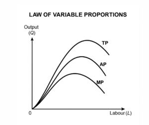
Three Stages of Production

Stage	Behaviour of Output	Economic Meaning
Stage I – Increasing Returns	TP and MP rise rapidly	Underutilization of fixed factor
Stage II – Diminishing Returns	TP rises at decreasing rate	Optimal production zone
Stage III – Negative Returns	TP declines; MP negative	Overcrowding of variable input

6. Isoquant Analysis (Long-Run Production)

Isoquant

An isoquant curve represents combinations of two inputs (labour and capital) yielding the same level of output.
It is analogous to an indifference curve in consumer theory.

Properties of Isoquants

Downward sloping: To maintain output, more of one input requires less of the other.
Convex to origin: Reflects diminishing Marginal Rate of Technical Substitution (MRTS).
Do not intersect: Each represents distinct output level.
Higher isoquants: Indicate higher output levels.

$M R T S_{L K} = - \frac{d K}{d L} = \frac{M P_{L}}{M P_{K}}$

Iso-Cost Line

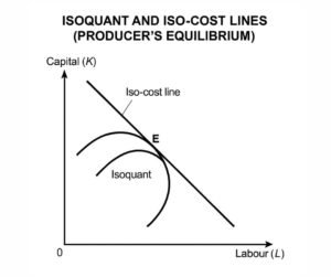
Represents all input combinations a firm can buy for a given cost:

$C = w L + r K$

Where $w$ = wage rate and $r$ = rental rate of capital.
Slope = -w/r

Producer’s Equilibrium

Occurs where the isoquant is tangent to an iso-cost line:

$\frac{M P_{L}}{M P_{K}} = \frac{w}{r}$

This represents the least-cost combination of inputs.

7. Returns to Scale (Long Run)

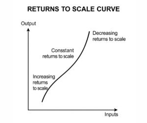
Examines how output responds to a proportionate change in all inputs.

Type	Description	Example
Increasing Returns to Scale (IRS)	Output increases more than proportionally.	Inputs ↑ 100% → Output ↑ > 100%
Constant Returns to Scale (CRS)	Output increases proportionally.	Inputs ↑ 100% → Output ↑ 100%
Decreasing Returns to Scale (DRS)	Output increases less than proportionally.	Inputs ↑ 100% → Output ↑ < 100%

Determinants of Returns to Scale

Indivisibility of inputs (e.g., machinery)
Specialization and division of labour
Managerial and technical efficiencies
Coordination challenges (for decreasing returns)

8. Theory of Costs

Cost refers to the expenditure incurred in producing goods and services.
It links production theory with financial decision-making.

Types of Costs

Cost Type	Definition	Example
Explicit (Actual)	Direct payments for inputs	Wages, rent, raw materials
Implicit (Imputed)	Value of self-owned resources	Owner’s labour, capital
Business Costs	Explicit + depreciation	Operational cost
Full Costs	Business + opportunity + normal profit	Economic cost
Out-of-Pocket	Cash payments	Wages, transport
Book Costs	Non-cash, accounting	Depreciation
Fixed Costs (TFC)	Remain constant with output	Rent, salaries
Variable Costs (TVC)	Vary with output	Raw materials, wages

Cost Functions

$T C = T F C + T V C$ $A C = \frac{T C}{Q}$ $M C = T C (n) - T C (n - 1)$

Relationships:

When MC < AC → AC falls
When MC > AC → AC rises
MC intersects AC at its minimum point

9. Cost Curves

Short-Run Cost Curves

AFC decreases continuously.
AVC and ATC are U-shaped due to economies and diseconomies of scale.
MC cuts both AVC and ATC at their minimum points.

Long-Run Cost Curves

All costs are variable.
LAC is the envelope of SRACs.
Traditionally U-shaped: reflects economies → constant returns → diseconomies of scale.

Modern (L-Shaped) Long-Run Cost Curve

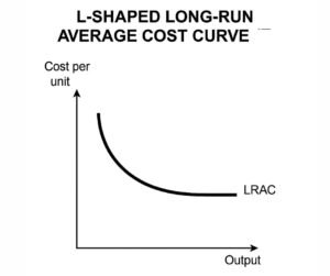
Empirical evidence shows costs flatten out at high output.
Due to:
- Reserve capacity of plants
- Learning curve and technical improvement
- Economies persisting at large scale

10. Economies and Diseconomies of Scale

Economies	Diseconomies
Internal: technical, managerial, marketing, financial, risk spreading	Managerial inefficiency, coordination failure, communication delays
External: industry growth, localization, shared infrastructure	Resource scarcity, input price rise

11. Relationship Between Production and Cost

$M C = \frac{w}{M P_{L}}$

As Marginal Product rises → Marginal Cost falls.
When MP falls → MC rises.
Thus, productivity curves and cost curves are mirror images.

12. Private and Social Costs

Type	Meaning
Private Cost	Costs borne by the firm itself.
Social Cost	Private + external costs (e.g., pollution, congestion).

13. Key Definitions

Term	Definition
Isoquant	Curve showing input combinations yielding same output
MRTS	Rate of technical substitution between inputs
Fixed Cost	Cost that does not vary with output in short run
Marginal Cost	Cost of producing one additional unit
Economies of Scale	Cost advantages from larger scale
Social Cost	Total cost to society (private + external)

14. Important Graphs

1️⃣ Law of Variable Proportions
2️⃣ Isoquant–Iso-Cost Tangency (Producer’s Equilibrium)
3️⃣ Returns to Scale Curve
4️⃣ L-shaped Long-Run Average Cost Curve

(Refer to the attached academic diagrams page for illustration.)

15. Summary Table for UGC NET

Concept	Focus	Key Relation
Short-Run Law	Variable proportions	TP, MP, AP behaviour
Long-Run Law	Returns to scale	IRS, CRS, DRS
Isoquant Analysis	Producer equilibrium	$M P_{L} / M P_{K} = w / r$
Cost Analysis	U and L-shaped curves	MC–AC interaction
Scale Effects	Economies vs. Diseconomies	Internal & External

UGC NET Economics Unit 1-Theory of Production and Costs

(Unit 1 – Microeconomics | UGC NET Economics)

1. Introduction

2. Classification of Inputs